顾名思义,所有的生物种群都是由个体集合而成的,因此会表现出一些新出现的特性,这些特性部分地概括了这些种群的特性。鉴于目前正在发生的许多物种灭绝事件,我同意,一个物种中的少数甚至单个个体可能会构成 “种群(population)”的某种限制,但我们将只关注更丰富的种群,而撇开这些可悲的极端情况。在这里,我们将重点关注个体的生长、成熟和补充,所有这些都与种群的生产力有关。与生长快、成熟早、繁殖力高的物种相比,生长慢、成熟晚、繁殖力低的物种的生产力往往较低,尽管其潜在稳定性更高。生命史特征的进化是一个复杂而又引人入胜的课题,我建议大家对其进行研究 (Beverton 和 Holt 1993; S. C. Stearns 1977; S. Stearns 1992)。不过,在这里我们将重点讨论简单得多的模型。即便如此,在对捕捞种群进行建模时,了解相关物种的生命史特征可能产生的影响,对于解释观察到的动态变化还是很有帮助的。不要忘记,生物过程建模极大地受益于生物知识和理解。
#vB growth curve fit to Pitcher and Macdonald derived seasonal data data(minnow); week<-minnow$week; length<-minnow$lengthpars<-c(75,0.1,-10.0,3.5); label=c("Linf","K","t0","sigma")bestvB<-nlm(f=negNLL,p=pars,funk=vB,ages=week,observed=length, typsize=magnitude(pars))predL<-vB(bestvB$estimate,0:160)outfit(bestvB,backtran =FALSE,title="Non-Seasonal vB",parnames=label)
nlm solution:  Non-Seasonal vB
minimum     :  150.6117
iterations  :  41
code        :  3 Either ~local min or steptol too small
                par      gradient
Linf   89.447640823  5.878821e-05
K       0.009909338  2.705709e-01
t0    -16.337065207 -4.717809e-05
sigma   3.741419172  2.711355e-04
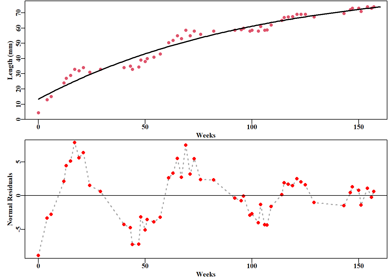
#plot the non-seasonal fit and its residuals. Figure 5.1 parset(plots=c(2,1),margin=c(0.35,0.45,0.02,0.05))plot1(week,length,type="p",cex=1.0,col=2,xlab="Weeks",pch=16, ylab="Length (mm)",defpar=FALSE)lines(0:160,predL,lwd=2,col=1)# calculate and plot the residuals resids<-length-vB(bestvB$estimate,week)plot1(week,resids,type="l",col="darkgrey",cex=0.9,lwd=2, xlab="Weeks",lty=3,ylab="Normal Residuals",defpar=FALSE)points(week,resids,pch=16,cex=1.1,col="red")abline(h=0,col=1,lwd=1)
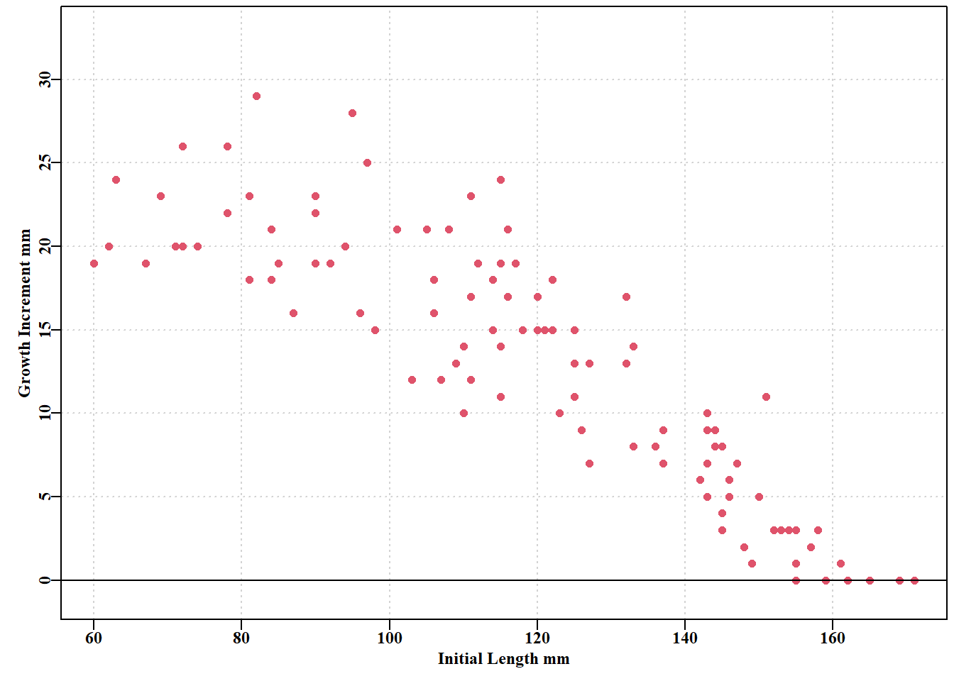
# tagging growth increment data from Black Island, Tasmania data(blackisland); bi<-blackisland# just to keep things brief parset()plot(bi$l1,bi$dl,type="p",pch=16,cex=1.0,col=2,ylim=c(-1,33), ylab="Growth Increment mm",xlab="Initial Length mm", panel.first =grid())abline(h=0,col=1)
# Fit the vB and Inverse Logistic to the tagging data linm<-lm(bi$dl~bi$l1)# simple linear regression param<-c(170.0,0.3,4.0); label<-c("Linf","K","sigma")modelvb<-nlm(f=negNLL,p=param,funk=fabens,observed=bi$dl,indat=bi, initL="l1",delT="dt")# could have used the defaults outfit(modelvb,backtran =FALSE,title="vB",parnames=label)
nlm solution:  vB
minimum     :  291.1691
iterations  :  24
code        :  1 gradient close to 0, probably solution
              par     gradient
Linf  173.9677972 9.563666e-07
K       0.2653003 2.656839e-04
sigma   3.5861240 1.391768e-05
nlm solution:  IL
minimum     :  277.0122
iterations  :  26
code        :  1 gradient close to 0, probably solution
            par      gradient
MaxDL  21.05654 -2.021972e-06
L50   130.92643  5.900276e-07
delta  40.98771  2.218945e-07
sigma   3.14555  4.535835e-06
代码
predil<-invl(modelil$estimate,bi)
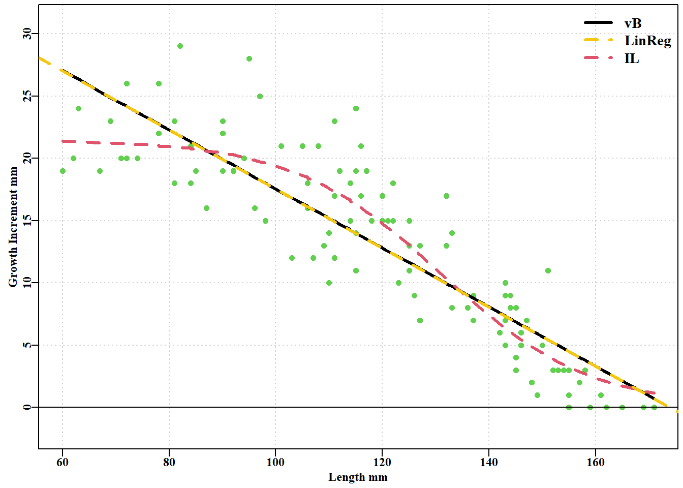
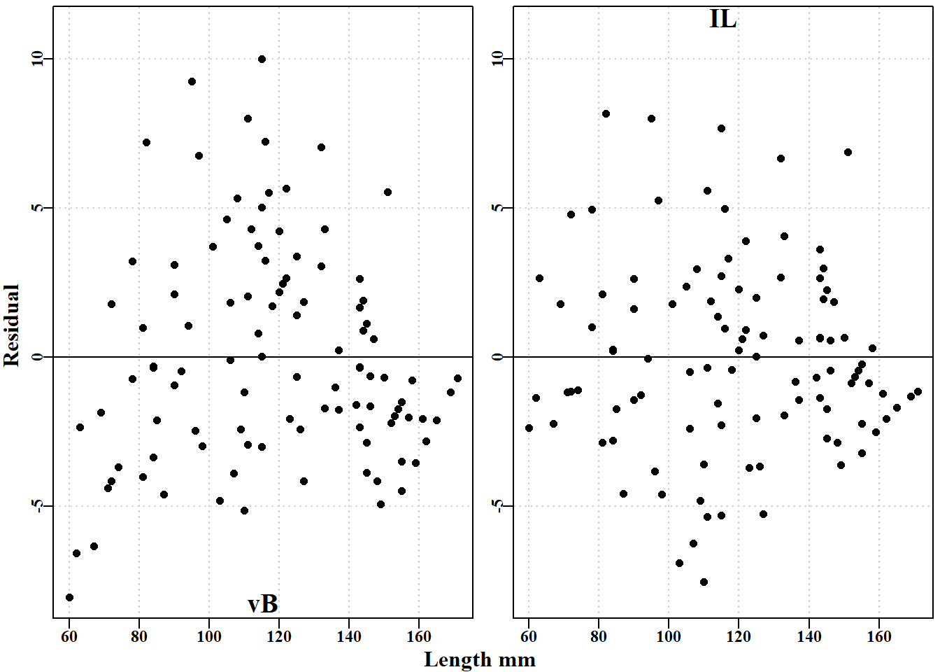
逆 logistic 模型的负对数似然小于 von Bertalanffy 模型的负对数似然,而且逆 logistic 呈现出较小的 \(\sigma\) 值。如果我们将这两条增长曲线与原始数据进行对比,就可以更清楚地看到它们之间的差异图 5.4。此外,对各自的残差进行检验也会发现曲线之间的差异,预测的 von Bertalanffy 曲线的残差呈圆弧状,这与其预测的初始长度与生长增量之间的线性关系是一致的。在 图 5.4 中,线性回归绘制在 von Bertalanffy 曲线的上方,以说明它实际上是重合的。
代码
#growth curves and regression fitted to tagging data Fig 5.4 parset(margin=c(0.4,0.4,0.05,0.05))plot(bi$l1,bi$dl,type="p",pch=16,cex=1.0,col=3,ylim=c(-2,31), ylab="Growth Increment mm",xlab="Length mm",panel.first=grid())abline(h=0,col=1)lines(bi$l1,predvB,pch=16,col=1,lwd=3,lty=1)# vB lines(bi$l1,predil,pch=16,col=2,lwd=3,lty=2)# IL abline(linm,lwd=3,col=7,lty=2)# add dashed linear regression legend("topright",c("vB","LinReg","IL"),lwd=3,bty="n",cex=1.2, col=c(1,7,2),lty=c(1,2,2))
#residuals for vB and inverse logistic for tagging data Fig 5.5 parset(plots=c(1,2),outmargin=c(1,1,0,0),margin=c(.25,.25,.05,.05))plot(bi$l1,(bi$dl-predvB),type="p",pch=16,col=1,ylab="", xlab="",panel.first=grid(),ylim=c(-8,11))abline(h=0,col=1)mtext("vB",side=1,outer=FALSE,line=-1.1,cex=1.2,font=7)plot(bi$l1,(bi$dl-predil),type="p",pch=16,col=1,ylab="", xlab="",panel.first=grid(),ylim=c(-8,11))abline(h=0,col=1)mtext("IL",side=3,outer=FALSE,line=-1.2,cex=1.2,font=7)mtext("Length mm",side=1,line=-0.1,cex=1.0,font=7,outer=TRUE)mtext("Residual",side=2,line=-0.1,cex=1.0,font=7,outer=TRUE)
# fit the Fabens tag growth curve with and without the option to # modify variation with predicted length. See the MQMF function # negnormL. So first no variation and then linear variation. sigfunk<-function(pars,predobs)return(tail(pars,1))#no effect data(blackisland)bi<-blackisland# just to keep things brief param<-c(170.0,0.3,4.0); label=c("Linf","K","sigma")modelvb<-nlm(f=negnormL,p=param,funk=fabens,funksig=sigfunk, indat=bi,initL="l1",delT="dt")outfit(modelvb,backtran =FALSE,title="vB constant sigma", parnames =label)
nlm solution:  vB constant sigma
minimum     :  291.1691
iterations  :  24
code        :  1 gradient close to 0, probably solution
              par     gradient
Linf  173.9677972 9.563666e-07
K       0.2653003 2.656839e-04
sigma   3.5861240 1.391768e-05
代码
sigfunk2<-function(pars,predo){# linear with predicted length sig<-tail(pars,1)*predo# sigma x predDL, see negnormL pick<-which(sig<=0)# ensure no negative sigmas from sig[pick]<-0.01# possible negative predicted lengths return(sig)}# end of sigfunk2 param<-c(170.0,0.3,1.0); label=c("Linf","K","sigma")modelvb2<-nlm(f=negnormL,p=param,funk=fabens,funksig=sigfunk2, indat=bi,initL="l1",delT="dt", typsize=magnitude(param),iterlim=200)outfit(modelvb2,backtran =FALSE,parnames =label, title="vB inverse DeltaL, sigma < 1")
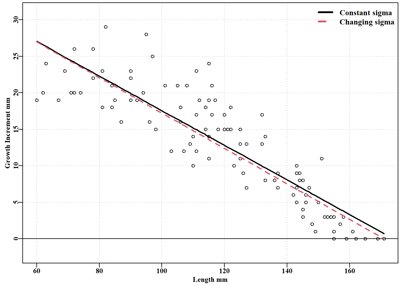
请记住,通过改变残差结构,似然值变得不相称,因此我们无法确定哪种拟合效果更好。恒定方差使得 von Bertalanffy 曲线在长度大于 148 左右时有效地保持在数据之上,而变化方差生长曲线大部分时间仍在数据之上,但由于方差随预测长度的减少而向后推近数据。我们可以通过重写 negnormL() 来进行实验,使用初始长度而不是预测长度。如前所述,将平均预测长度与相关方差分离可以获得极大的灵活性。
代码
#plot to two Faben's lines with constant and varying sigma Fig 5.6 predvB<-fabens(modelvb$estimate,bi)predvB2<-fabens(modelvb2$estimate,bi)parset(margin=c(0.4,0.4,0.05,0.05))plot(bi$l1,bi$dl,type="p",pch=1,cex=1.0,col=1,ylim=c(-2,31), ylab="Growth Increment mm",xlab="Length mm",panel.first=grid())abline(h=0,col=1)lines(bi$l1,predvB,col=1,lwd=2)# vB lines(bi$l1,predvB2,col=2,lwd=2,lty=2)# IL legend("topright",c("Constant sigma","Changing sigma"),lwd=3, col=c(1,2),bty="n",cex=1.1,lty=c(1,2))
图 5.6: 与黑岛黑唇鲍标记数据拟合的具有恒定 sigma von Bertalanffy(皇家蓝)和 具有与不断变化的 DeltaL 相关的 sgima 的 von Bertalanffy(红色虚线)。 标记与再捕之间的平均时间间隔为 1.02 年。
关于 von Bertalanffy 曲线和逆逻辑斯蒂曲线的比较,逆逻辑斯蒂负对数似然值为 \(-2.0 \times(277.0122-291.1691) = 28.3138\) ,明显小于 von Bertalanffy 曲线的负对数似然值。我们可以使用 MQMF 函数 likeratio()来说明这两种曲线在拟合数据方面的差异具有高度显著性。
代码
# Likelihood ratio comparison of two growth models see Fig 5.4 vb<-modelvb$minimum# their respective -ve log-likelihoods il<-modelil$minimumdof<-1round(likeratio(vb,il,dof),8)
         LR           P      mindif          df
28.31380340  0.00000005  3.84145882  1.00000000
# The Maturity data from tasab data-set data(tasab)# see ?tasab for a list of the codes used properties(tasab)# summarize properties of columns in tasab
       Index isNA Unique     Class Min Max Example
site       1    0      2   integer   1   2       1
sex        2    0      3 character   0   0       I
length     3    0     85   integer  62 160     102
mature     4    0      2   integer   0   1       0
代码
table(tasab$site,tasab$sex)# sites 1 & 2 vs F, I, and M
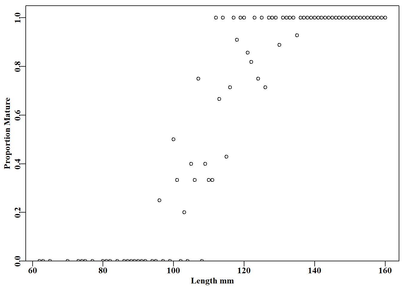
#plot the proportion mature vs shell length Fig 5.7 propm<-tapply(tasab$mature,tasab$length,mean)#mean maturity at L lens<-as.numeric(names(propm))# lengths in the data plot1(lens,propm,type="p",cex=0.9,xlab="Length mm", ylab="Proportion Mature")
#Use glm to estimate mature logistic binglm<-function(x,digits=6){#function to simplify printing out<-summary(x)print(out$call)print(round(out$coefficients,digits))cat("\nNull Deviance ",out$null.deviance,"df",out$df.null,"\n")cat("Resid.Deviance ",out$deviance,"df",out$df.residual,"\n")cat("AIC = ",out$aic,"\n\n")return(invisible(out))# retain the full summary }#end of binglm tasab$site<-as.factor(tasab$site)# site as a factor smodel<-glm(mature~site+length,family=binomial,data=tasab)outs<-binglm(smodel)#outs contains the whole summary object
glm(formula = mature ~ site + length, family = binomial, data = tasab)
              Estimate Std. Error   z value Pr(>|z|)
(Intercept) -19.797096   2.361561 -8.383056 0.000000
site2        -0.369502   0.449678 -0.821703 0.411246
length        0.182551   0.019872  9.186463 0.000000

Null Deviance   564.0149 df 714
Resid.Deviance  170.7051 df 712
AIC  =  176.7051
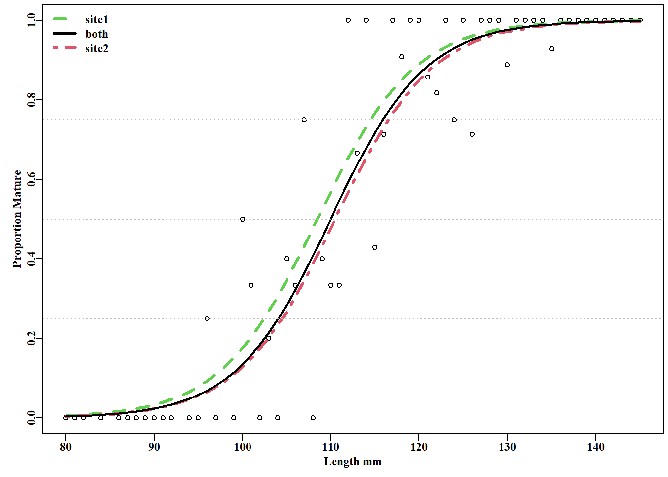
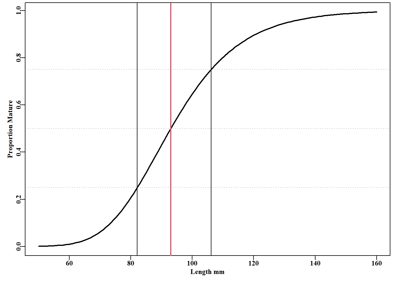
#Add maturity logistics to the maturity data plot Fig 5.8 propm<-tapply(tasab$mature,tasab$length,mean)#prop mature lens<-as.numeric(names(propm))# lengths in the data pick<-which((lens>79)&(lens<146))parset()plot(lens[pick],propm[pick],type="p",cex=0.9, #the data points xlab="Length mm",ylab="Proportion Mature",pch=1)L<-seq(80,145,1)# for increased curve separation pars<-coef(smodel)lines(L,mature(pars[1],pars[3],L),lwd=3,col=3,lty=2)lines(L,mature(pars[1]+pars[2],pars[3],L),lwd=3,col=2,lty=4)lines(L,mature(coef(model)[1],coef(model)[2],L),lwd=2,col=1,lty=1)abline(h=c(0.25,0.5,0.75),lty=3,col="grey")legend("topleft",c("site1","both","site2"),col=c(3,1,2),lty=c(2,1,4), lwd=3,bty="n")
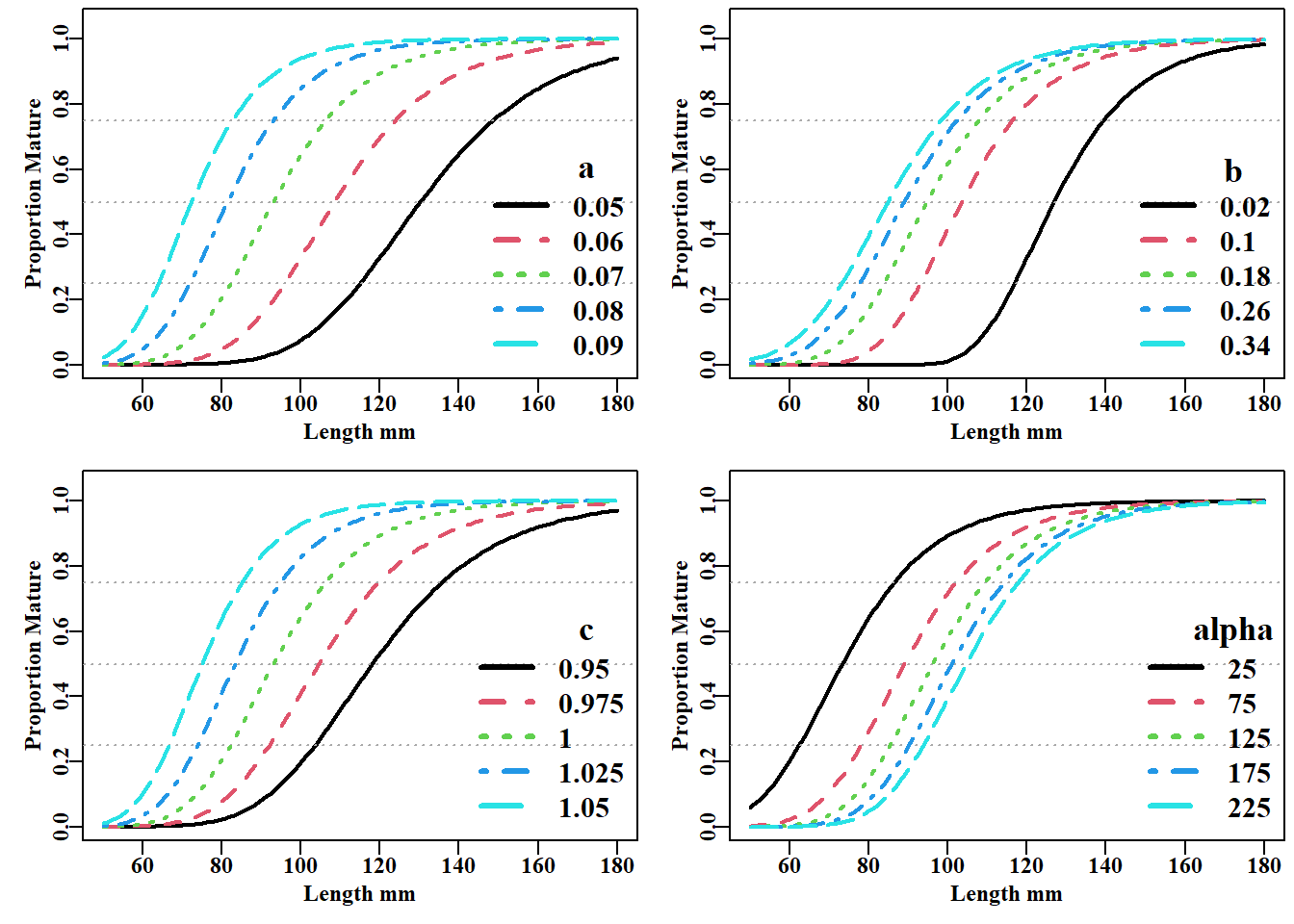
#Variation possible using the Schnute and Richard's Curve fig 5.10 # This code not printed in the book tmplot<-function(vals,label){text(170,0.6,paste0(" ",label),font=7,cex=1.5)legend("bottomright",legend=vals,col=1:nvals,lwd=3,bty="n", cex=1.25,lty=c(1:nvals))}L=seq(50,180,1)vals<-seq(0.05,0.09,0.01)# a value nvals<-length(vals)asym<-srug(p=c(a=vals[1],b=0.2,c=1.0,alpha=100),sizeage=L)oldp<-parset(plots=c(2,2))plot(L,asym,type="l",lwd=2,xlab="Length mm",ylab="Proportion Mature", ylim=c(0,1.05))abline(h=c(0.25,0.5,0.75),lty=3,col="darkgrey")for(iin2:nvals){asym<-srug(p=c(a=vals[i],b=0.2,c=1.0,alpha=100),sizeage=L)lines(L,asym,lwd=2,col=i,lty=i)}tmplot(vals,"a")vals<-seq(0.02,0.34,0.08)# b value nvals<-length(vals)asym<-srug(p=c(a=0.07,b=vals[1],c=1.0,alpha=100),sizeage=L)plot(L,asym,type="l",lwd=2,xlab="Length mm",ylab="Proportion Mature", ylim=c(0,1.05))abline(h=c(0.25,0.5,0.75),lty=3,col="darkgrey")for(iin2:nvals){asym<-srug(p=c(a=0.07,b=vals[i],c=1.0,alpha=100),sizeage=L)lines(L,asym,lwd=2,col=i,lty=i)}tmplot(vals,"b")vals<-seq(0.95,1.05,0.025)# c value nvals<-length(vals)asym<-srug(p=c(a=0.07,b=0.2,c=vals[1],alpha=100),sizeage=L)plot(L,asym,type="l",lwd=2,xlab="Length mm",ylab="Proportion Mature", ylim=c(0,1.05))abline(h=c(0.25,0.5,0.75),lty=3,col="darkgrey")for(iin2:nvals){asym<-srug(p=c(a=0.07,b=0.2,c=vals[i],alpha=100),sizeage=L)lines(L,asym,lwd=2,col=i,lty=i)}tmplot(vals,"c")vals<-seq(25,225,50)# alpha value nvals<-length(vals)asym<-srug(p=c(a=0.07,b=0.2,c=1.0,alpha=vals[1]),sizeage=L)plot(L,asym,type="l",lwd=2,xlab="Length mm",ylab="Proportion Mature", ylim=c(0,1.05))abline(h=c(0.25,0.5,0.75),lty=3,col="darkgrey")for(iin2:nvals){asym<-srug(p=c(a=0.07,b=0.2,c=1.0,alpha=vals[i]),sizeage=L)lines(L,asym,lwd=2,col=i,lty=i)}tmplot(vals,"alpha")par(oldp)# return par to old settings; this line not in book
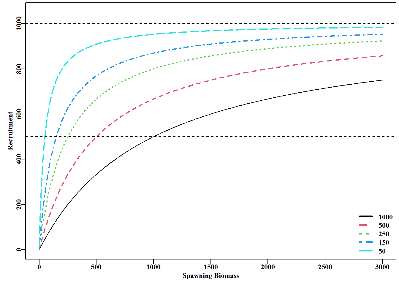
#plot the MQMF bh function for Beverton-Holt recruitment Fig 5.11 B<-1:3000bhb<-c(1000,500,250,150,50)parset()plot(B,bh(c(1000,bhb[1]),B),type="l",ylim=c(0,1050), xlab="Spawning Biomass",ylab="Recruitment")for(iin2:5)lines(B,bh(c(1000,bhb[i]),B),lwd=2,col=i,lty=i)legend("bottomright",legend=bhb,col=c(1:5),lwd=3,bty="n",lty=c(1:5))abline(h=c(500,1000),col=1,lty=2)
图 5.11: 有恒定 a = 1000 和五个递减的 b 值的Beverton-Holt 种群补充曲线,导致越来越高效的曲线。
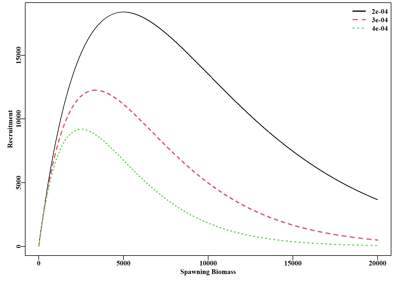
#plot the MQMF ricker function for Ricker recruitment Fig 5.12 B<-1:20000rickb<-c(0.0002,0.0003,0.0004)parset()plot(B,ricker(c(10,rickb[1]),B),type="l",xlab="Spawning Biomass", ylab="Recruitment")for(iin2:3)lines(B,ricker(c(10,rickb[i]),B),lwd=2,col=i,lty=i)legend("topright",legend=rickb,col=1:3,lty=1:3,bty="n",lwd=2)
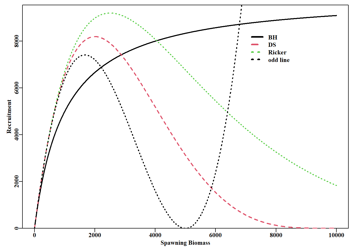
# plot of three special cases from Deriso-Schnute curve Fig. 5.13 deriso<-function(p,B)return(p[1]*B*(1-p[2]*p[3]*B)^(1/p[3]))B<-1:10000plot1(B,deriso(c(10,0.001,-1),B),lwd=2, xlab="Spawning Biomass",ylab="Recruitment")# BH lines(B,deriso(c(10,0.0004,0.25),B),lwd=2,col=2,lty=2)# DS lines(B,deriso(c(10,0.0004,1e-06),B),lwd=2,col=3,lty=3)# Ricker lines(B,deriso(c(10,0.0004,0.5),B),lwd=2,col=1,lty=3)# odd line legend(x=7000,y=8500,legend=c("BH","DS","Ricker","odd line"), col=c(1,2,3,1),lty=c(1,2,3,3),bty="n",lwd=3)
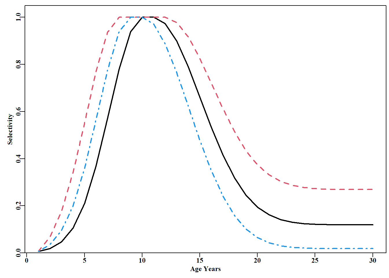
#Examples of domed-shaped selectivity curves from domed. Fig.5.15 L<-seq(1,30,1)p<-c(10,11,16,33,-5,-2)plot1(L,domed(p,L),type="l",lwd=2,ylab="Selectivity",xlab="Age Years")p1<-c(8,12,16,33,-5,-1)lines(L,domed(p1,L),lwd=2,col=2,lty=2)p2<-c(9,10,16,33,-5,-4)lines(L,domed(p2,L),lwd=2,col=4,lty=4)
Pitcher, T. J., 和 P. D. M. Macdonald. 1973. 《Two Models for Seasonal Growth in Fishes》. The Journal of Applied Ecology 10 (2): 599. https://doi.org/10.2307/2402304.
Stearns, SC. 1992. The evolution of life histories. Oxford University Press.
Stearns, Stephen C. 1977. 《The Evolution of Life History Traits: A Critique of the Theory and a Review of the Data》. Annual Review of Ecology and Systematics 8 (1): 145–71. https://doi.org/10.1146/annurev.es.08.110177.001045.