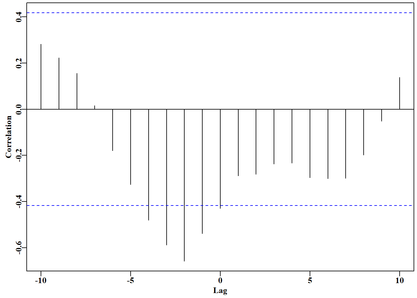
# cross correlation between cpue and catch in schaef Fig 7.2parset(cex =0.85)# sets par parameters for a tidy base graphicccf( x =schaef[, "catch"], y =schaef[, "cpue"], type ="correlation", ylab ="Correlation", plot =TRUE)
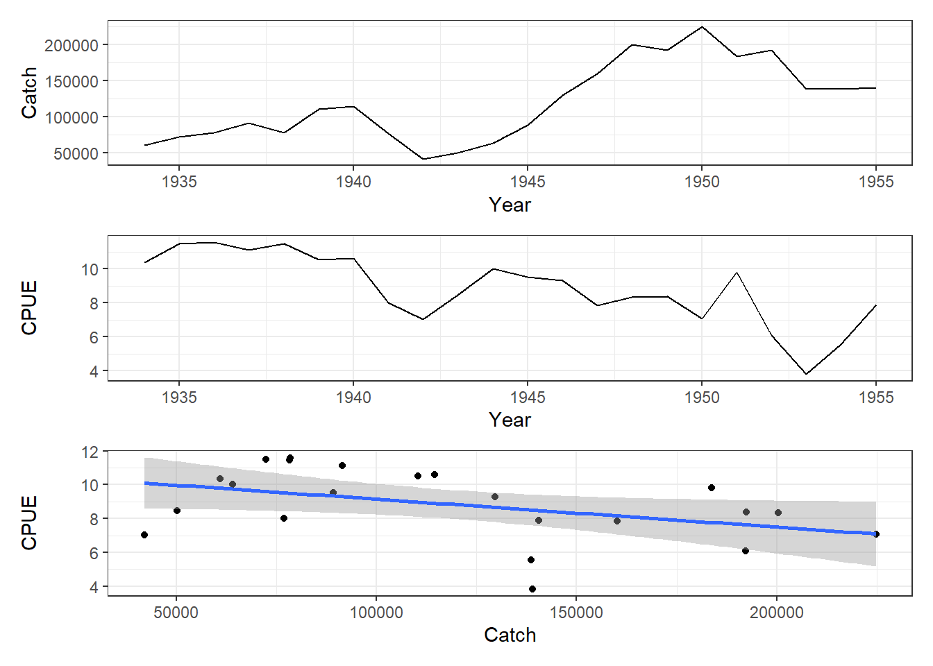
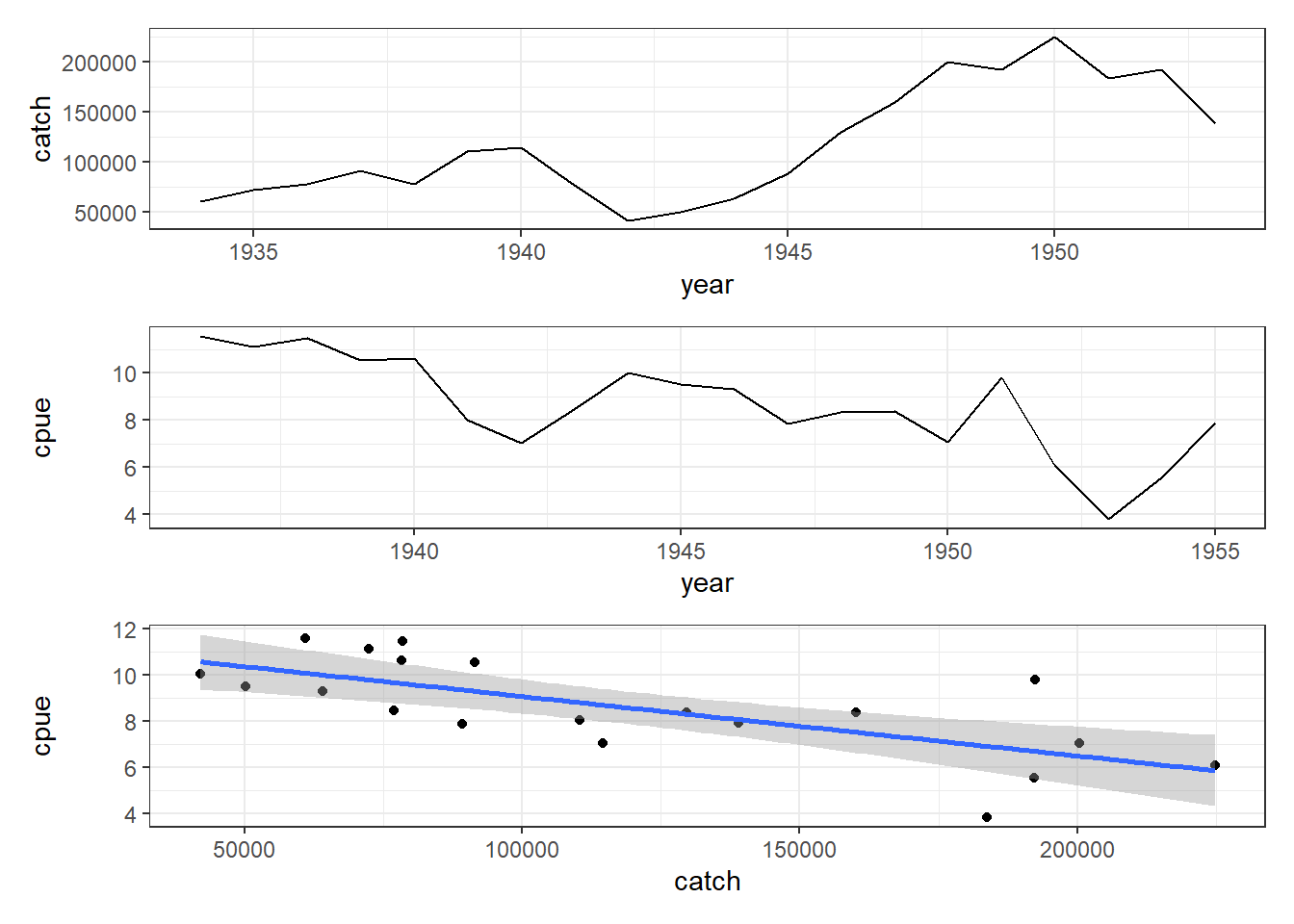
# now plot schaef data with timelag of 2 years on cpue Fig 7.3model2<-lm(schaef[3:22, "cpue"]~schaef[1:20, "catch"])# parset(plots=c(3,1),margin=c(0.35,0.4,0.05,0.05))# plot1(schaef[1:20,"year"],schaef[1:20,"catch"],ylab="Catch",# xlab="Year",defpar=FALSE,lwd=2)# plot1(schaef[3:22,"year"],schaef[3:22,"cpue"],ylab="CPUE",# xlab="Year",defpar=FALSE,lwd=2)# plot(schaef[1:20,"catch"],schaef[3:22,"cpue"],type="p",# ylab="CPUE",xlab="Catch",defpar=FALSE,cex=1.0,pch=16)## abline(model2,lwd=2,col=2)p1<-schaef|>filter(year<=1953)|>ggplot(aes(x =year, y =catch))+geom_line()+theme_bw()p2<-schaef|>filter(year>1935)|>ggplot(aes(x =year, y =cpue))+geom_line()+theme_bw()l<-nrow(schaef)schaef1<-data.frame( catch =schaef[1:(l-2), "catch"], cpue =schaef[3:l, "cpue"])p3<-ggplot(data =schaef1, aes(x =catch, y =cpue))+geom_point()+geom_smooth(method ="lm")+theme_bw()p1/p2/p3
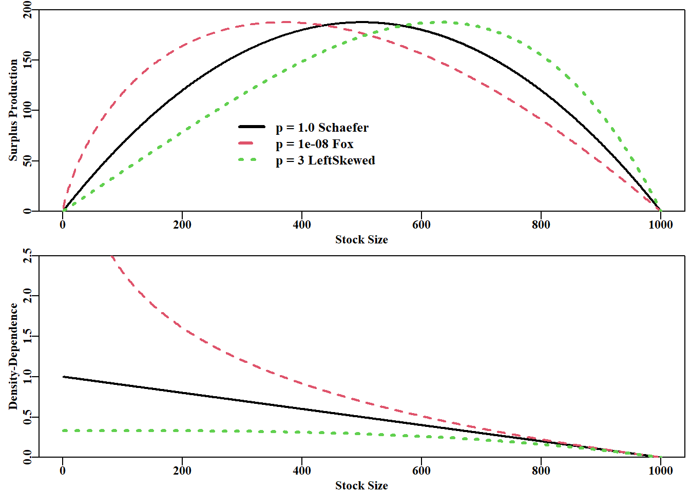
# compare Schaefer and Fox MSY estimates for same parametersparam<-c(r =1.1, K =1000.0, Binit =800.0, sigma =0.075)cat("MSY Schaefer = ", getMSY(param, p =1.0), "\n")# p=1 is default
# Fit the model first using optim then nlm in sequenceparam<-log(c(0.1, 2250000, 2250000, 0.5))pnams<-c("r", "K", "Binit", "sigma")best<-optim( par =param, fn =negLL, funk =simpspm, indat =schaef, logobs =log(schaef[, "cpue"]), method ="BFGS")outfit(best, digits =4, title ="Optim", parnames =pnams)
# the high-level structure of ans; try str(ans$Dynamics)str(ans, width =65, strict.width ="cut", max.level =1)
List of 12
 $ Dynamics :List of 5
 $ BiomProd : num [1:200, 1:2] 100 10687 21273 31860 42446 ...
  ..- attr(*, "dimnames")=List of 2
 $ rmseresid: num 1.03
 $ MSY      : num 123731
 $ Bmsy     : num 1048169
 $ Dmsy     : num 0.498
 $ Blim     : num 423562
 $ Btarg    : num 1016409
 $ Ctarg    : num 123581
 $ Dcurr    : Named num 0.528
  ..- attr(*, "names")= chr "1956"
 $ rmse     :List of 1
 $ sigma    : num 0.169
# conduct a robustness test on the Schaefer model fitdata(schaef)schaef<-as.matrix(schaef)reps<-12param<-log(c(r =0.15, K =2250000, Binit =2250000, sigma =0.5))ansS<-fitSPM( pars =param, fish =schaef, schaefer =TRUE, # use maxiter =1000, funk =simpspm, funkone =FALSE)# fitSPM# getseed() #generates random seed for repeatable resultsset.seed(777852)# sets random number generator with a known seedrobout<-robustSPM( inpar =ansS$estimate, fish =schaef, N =reps, scaler =40, verbose =FALSE, schaefer =TRUE, funk =simpspm, funkone =FALSE)# use str(robout) to see the components included in the output
表 7.2: A robustness test of the fit to the schaef data-set. By examining the results object we can see the individual variation. The top columns relate to the initial parameters and the bottom columns, perhaps of more interest, to the model fits.
# Repeat robustness test on fit to schaef data 100 timesset.seed(777854)robout2<-robustSPM( inpar =ansS$estimate, fish =schaef, N =100, scaler =25, verbose =FALSE, schaefer =TRUE, funk =simpspm, funkone =TRUE, steptol =1e-06)lastbits<-tail(robout2$results[, 6:11], 10)
表 7.3: The last 10 trials from the 100 illustrating that the last three trials deviated a little from the optimum negative log-likelihood of -7.93406.
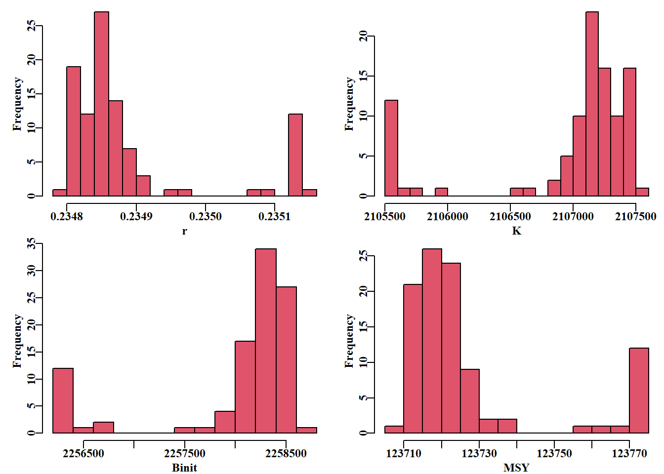
# replicates from the robustness test Fig 7.7result<-robout2$resultsparset(plots =c(2, 2), margin =c(0.35, 0.45, 0.05, 0.05))hist(result[, "r"], breaks =15, col =2, main ="", xlab ="r")hist(result[, "K"], breaks =15, col =2, main ="", xlab ="K")hist(result[, "Binit"], breaks =15, col =2, main ="", xlab ="Binit")hist(result[, "MSY"], breaks =15, col =2, main ="", xlab ="MSY")
# Now use the dataspm data-set, which is noisierset.seed(777854)# other random seeds give different resultsdata(dataspm)fish<-dataspm# to generalize the codeparam<-log(c(r =0.24, K =5174, Binit =2846, sigma =0.164))ans<-fitSPM( pars =param, fish =fish, schaefer =TRUE, maxiter =1000, funkone =TRUE)out<-robustSPM(ans$estimate, fish, N =100, scaler =15, # making verbose =FALSE, funkone =TRUE)# scaler=10 givesresult<-tail(out$results[, 6:11], 10)# 16 sub-optimal results
表 7.4: The last 10 trials from 100 used with dataspm. The last six trials deviate markedly from the optimum negative log-likelihood of -12.1288, and five gave consistent sub-optimal optima. Variation across parameter estimates with the optimum log-likelihood remained minor, but was large for the false optima.
当我们测试一些模型拟合对初始条件的稳健性时,我们发现当拟合多个参数时,可以从略微不同的参数值中获得基本相同的数值拟合(达到给定的精度)。虽然这些值往往相差不大,但这一观察结果仍然证实,当使用数值方法估计一组参数时,特定参数值并不是唯一重要的结果。我们还需要知道这些估计的精确程度,我们需要知道与它们的估计相关的任何不确定性。有许多方法可以用来探索模型拟合中的不确定性。在这里,我们将使用 R 检查四个的实现:1)似然剖面,2)自举重采样,3) 渐近误差,以及 4)贝叶斯后验分布。
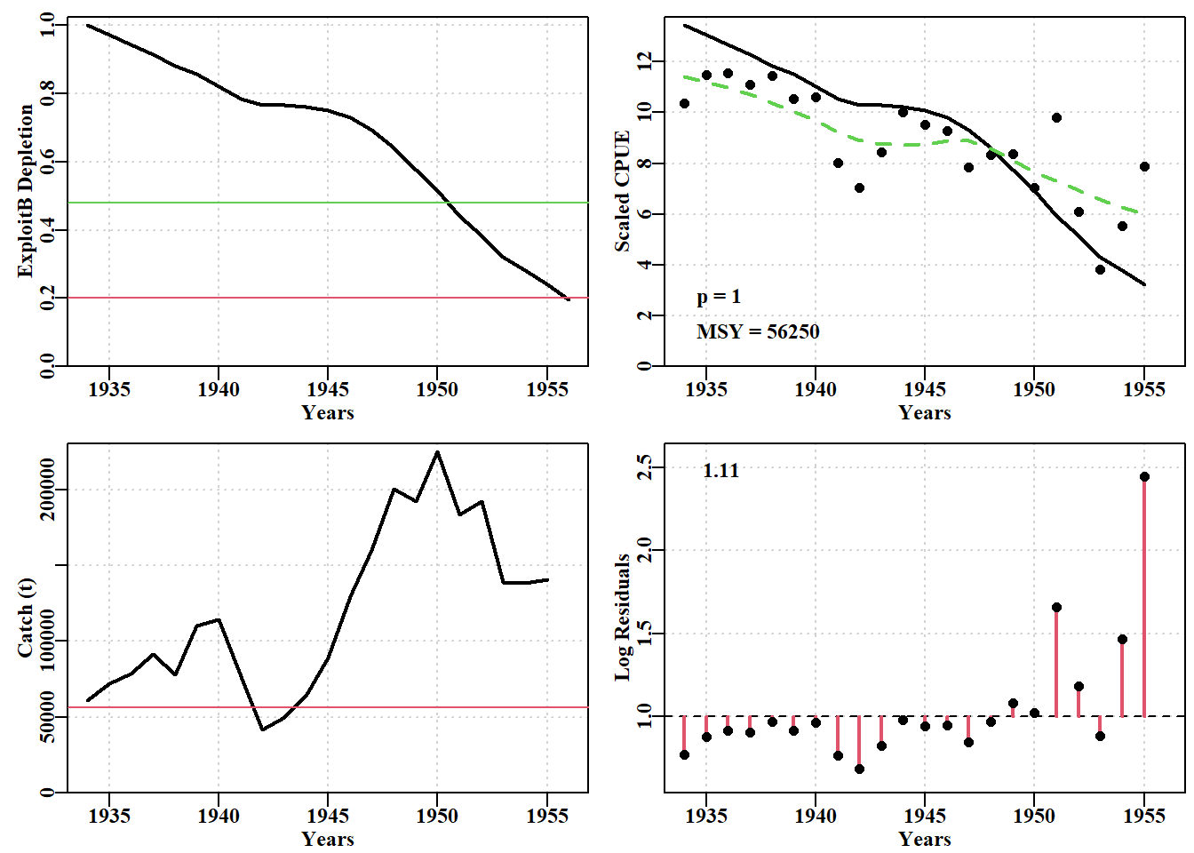
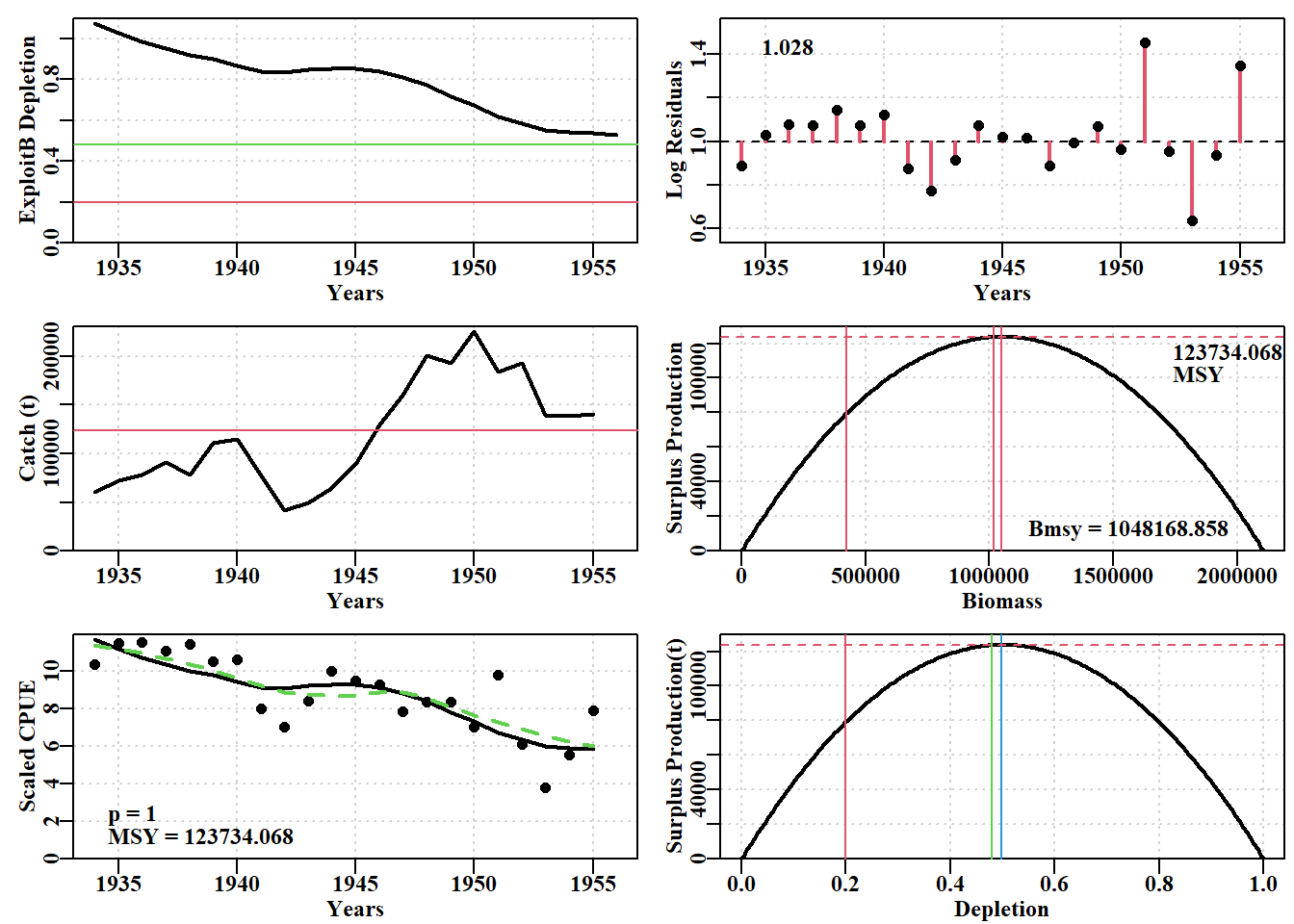
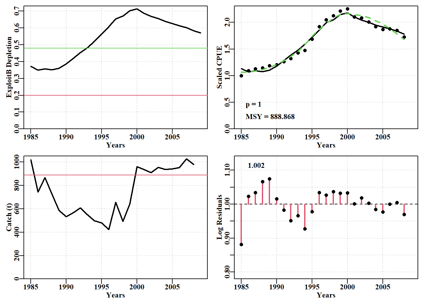
# Fig 7.9 Fit of optimum to the abdat data-setdata(abdat)fish<-as.matrix(abdat)colnames(fish)<-tolower(colnames(fish))# just in casepars<-log(c(r =0.4, K =9400, Binit =3400, sigma =0.05))ans<-fitSPM(pars, fish, schaefer =TRUE)# Schaeferanswer<-plotspmmod(ans$estimate, abdat, schaefer =TRUE, addrmse =TRUE)
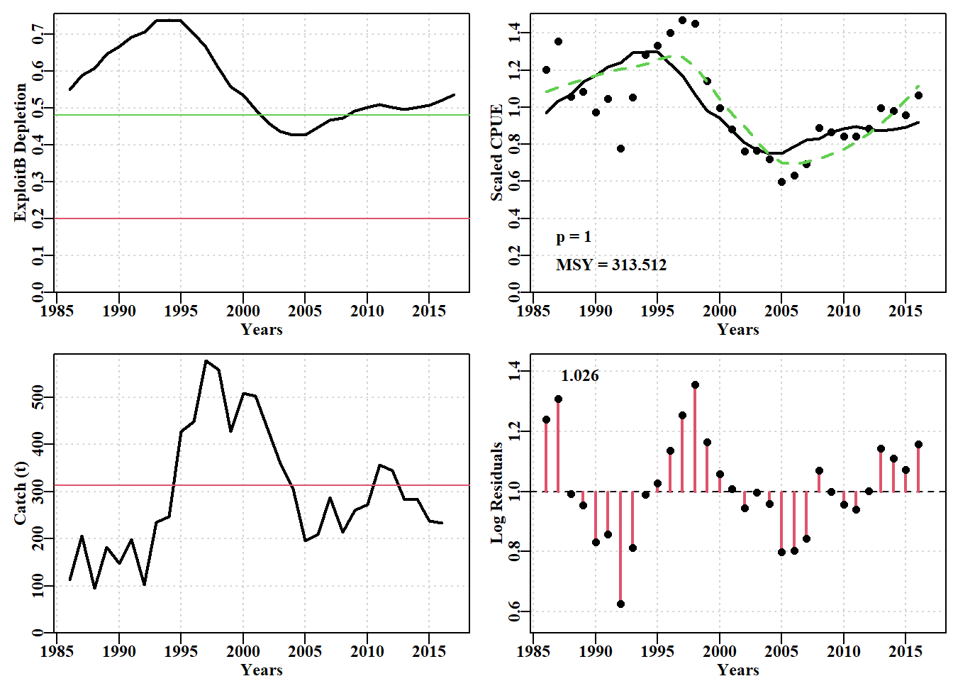
#find optimum Schaefer model fit to dataspm data-set Fig 7.11 data(dataspm)fish<-as.matrix(dataspm)colnames(fish)<-tolower(colnames(fish))pars<-log(c(r=0.25,K=5500,Binit=3000,sigma=0.25))ans<-fitSPM(pars,fish,schaefer=TRUE,maxiter=1000)#Schaefer answer<-plotspmmod(ans$estimate,fish,schaefer=TRUE,addrmse=TRUE)
#bootstrap the log-normal residuals from optimum model fit set.seed(210368)reps<-1000# can take 10 sec on a large Desktop. Be patient #startime <- Sys.time() # schaefer=TRUE is the default boots<-spmboot(ans$estimate,fishery=fish,iter=reps)#print(Sys.time() - startime) # how long did it take? str(boots,max.level=1)
List of 2
 $ dynam  : num [1:1000, 1:31, 1:5] 2846 3555 2459 3020 1865 ...
  ..- attr(*, "dimnames")=List of 3
 $ bootpar: num [1:1000, 1:8] 0.242 0.236 0.192 0.23 0.361 ...
  ..- attr(*, "dimnames")=List of 2
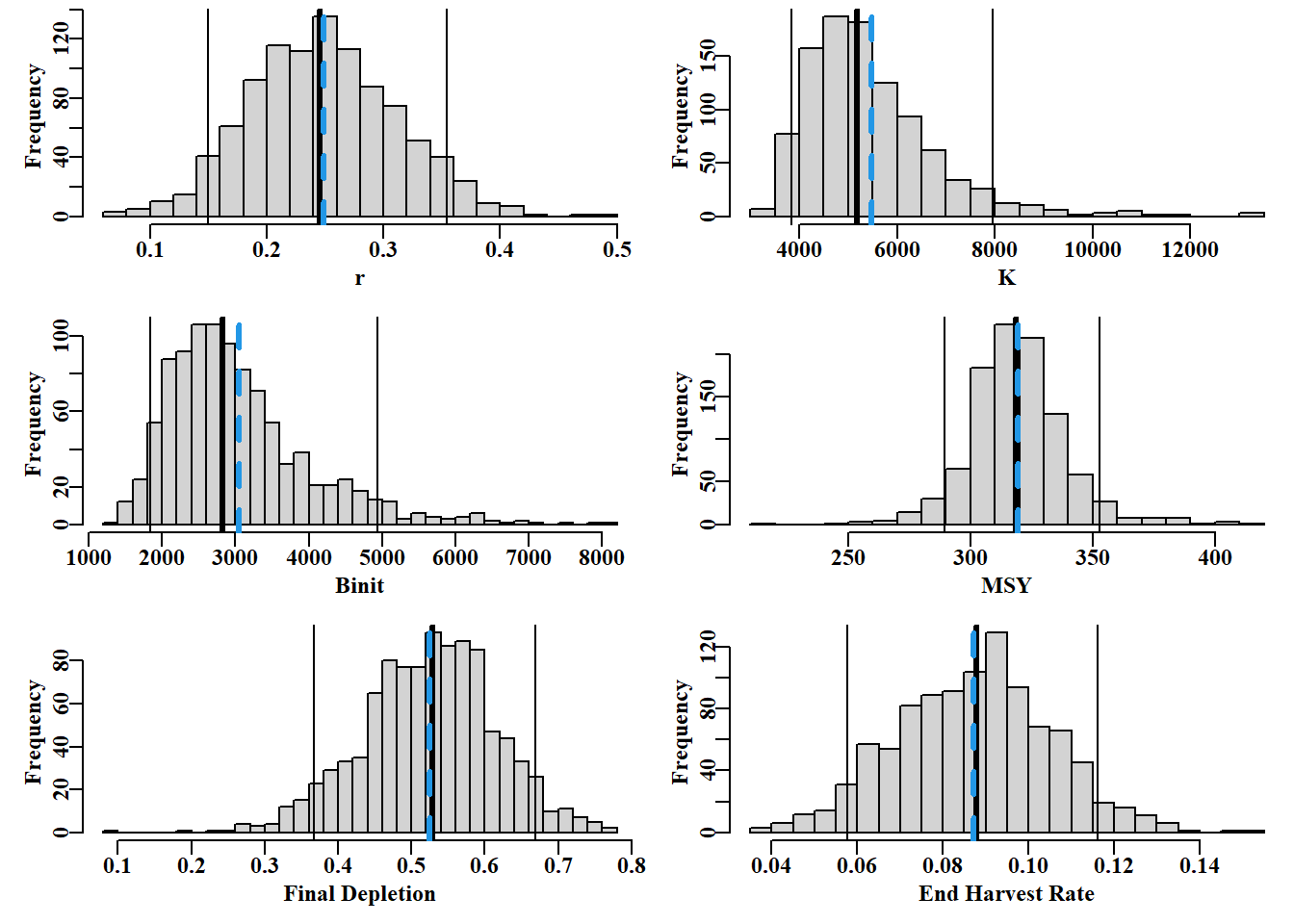
#boostrap CI. Note use of uphist to expand scale Fig 7.12 {colf<-c(1,1,1,4); lwdf<-c(1,3,1,3); ltyf<-c(1,1,1,2)colsf<-c(2,3,4,6)parset(plots=c(3,2))hist(bootpar[,"r"],breaks=25,main="",xlab="r")abline(v=c(bootCI["r",colsf]),col=colf,lwd=lwdf,lty=ltyf)uphist(bootpar[,"K"],maxval=14000,breaks=25,main="",xlab="K")abline(v=c(bootCI["K",colsf]),col=colf,lwd=lwdf,lty=ltyf)hist(bootpar[,"Binit"],breaks=25,main="",xlab="Binit")abline(v=c(bootCI["Binit",colsf]),col=colf,lwd=lwdf,lty=ltyf)uphist(bootpar[,"MSY"],breaks=25,main="",xlab="MSY",maxval=450)abline(v=c(bootCI["MSY",colsf]),col=colf,lwd=lwdf,lty=ltyf)hist(bootpar[,"Depl"],breaks=25,main="",xlab="Final Depletion")abline(v=c(bootCI["Depl",colsf]),col=colf,lwd=lwdf,lty=ltyf)hist(bootpar[,"Harv"],breaks=25,main="",xlab="End Harvest Rate")abline(v=c(bootCI["Harv",colsf]),col=colf,lwd=lwdf,lty=ltyf)}
图 7.12: The 1000 bootstrap replicates from the optimum spm fit to the dataspm data-set. The vertical lines, in each case, are the median and 90th percentile confidence intervals and the dashed vertical blue lines are the mean values. The function uphist() is used to expand the x-axis in K, Binit, and MSY.
存储在 boots$dynam 中的拟合轨迹也可以直观地指示分析的不确定性。
代码
#Fig7.13 1000 bootstrap trajectories for dataspm model fit dynam<-boots$dynamyears<-fish[,"year"]nyrs<-length(years)parset()ymax<-getmax(c(dynam[,,"predCE"],fish[,"cpue"]))plot(fish[,"year"],fish[,"cpue"],type="n",ylim=c(0,ymax), xlab="Year",ylab="CPUE",yaxs="i",panel.first =grid())for(iin1:reps)lines(years,dynam[i,,"predCE"],lwd=1,col=8)lines(years,answer$Dynamics$outmat[1:nyrs,"predCE"],lwd=2,col=0)points(years,fish[,"cpue"],cex=1.2,pch=16,col=1)percs<-apply(dynam[,,"predCE"],2,quants)arrows(x0=years,y0=percs["5%",],y1=percs["95%",],length=0.03, angle=90,code=3,col=0)
图 7.13: A plot of the original observed CPUE (black dots), the optimum predicted CPUE (solid line), the 1000 bootstrap predicted CPUE (the grey lines), and the 90th percentile confidence intervals around those predicted values (the vertical bars).
值得一做的是重复上述分析,但将 schaefer = TRUE 处改为 FALSE ,以便用 Fox 剩余产量模型来拟合模型。这样就可以比较两个模型的不确定性。
代码
#Fit the Fox model to dataspm; note different parameters pars<-log(c(r=0.15,K=6500,Binit=3000,sigma=0.20))ansF<-fitSPM(pars,fish,schaefer=FALSE,maxiter=1000)#Fox version bootsF<-spmboot(ansF$estimate,fishery=fish,iter=reps,schaefer=FALSE)dynamF<-bootsF$dynam
代码
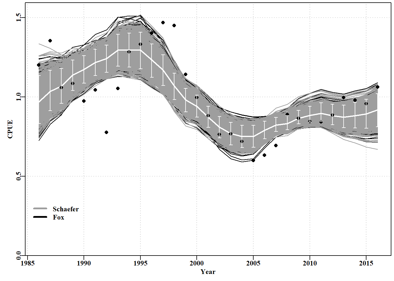
# bootstrap trajectories from both model fits Fig 7.14 parset()ymax<-getmax(c(dynam[,,"predCE"],fish[,"cpue"]))plot(fish[,"year"],fish[,"cpue"],type="n",ylim=c(0,ymax), xlab="Year",ylab="CPUE",yaxs="i",panel.first =grid())for(iin1:reps)lines(years,dynamF[i,,"predCE"],lwd=1,col=1,lty=1)for(iin1:reps)lines(years,dynam[i,,"predCE"],lwd=1,col=8)lines(years,answer$Dynamics$outmat[1:nyrs,"predCE"],lwd=2,col=0)points(years,fish[,"cpue"],cex=1.1,pch=16,col=1)percs<-apply(dynam[,,"predCE"],2,quants)arrows(x0=years,y0=percs["5%",],y1=percs["95%",],length=0.03, angle=90,code=3,col=0)legend(1985,0.35,c("Schaefer","Fox"),col=c(8,1),bty="n",lwd=3)
图 7.14: A plot of the original observed CPUE (dots), the optimum predicted CPUE (solid white line) with the 90th percentile confidence intervals (the white bars). The black lines are the Fox model bootstrap replicates while the grey lines over the black are those from the Schaefer model.
可以说,Fox 模型在捕捉这些数据的变异性方面更成功,因为黑线的扩散范围略大于灰色线(图 7.14)。或者,可以说 Fox 模型不太确定。总体而言,Schaefer 和 Fox 模型的输出之间没有太大差异,甚至像他们预测的那样 \(MSY\) 值非常相似(313.512 吨与 311.661 吨)。然而,最终,Fox 模型中密度依赖性的非线性似乎赋予了它更大的灵活性,因此它能够比更严格的 Schaefer 模型更好地捕获原始数据的变异性(因此它的 -ve 对数似然性更小,参见 outfit(ansF))。但这两个模型都无法捕获残差中表现出的循环特性,意味着建模动力学中未包含某些过程,即模型错误规范。这两种模型都不完全充分,尽管它们都可以提供足够的近似动态,可以用来产生管理建议(关于周期过程随时间保持不变的警告,等等)。
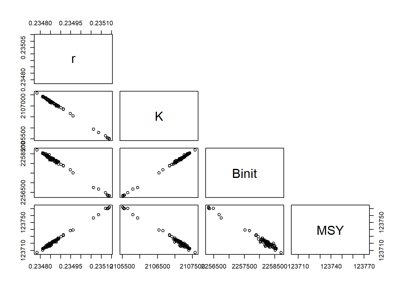
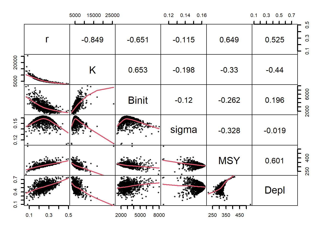
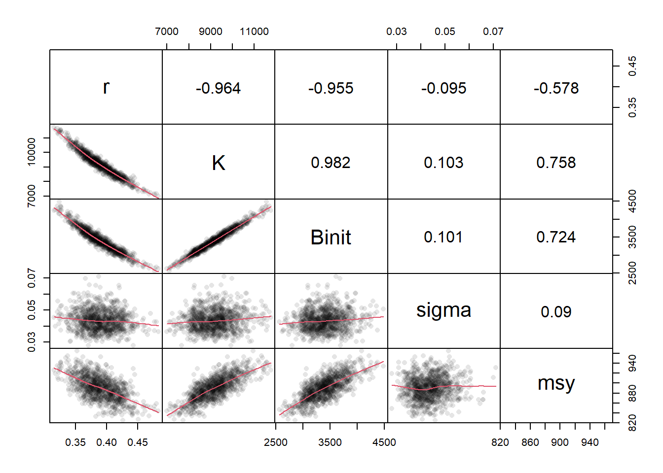
 # plot variables against each other, use MQMF panel.cor  Fig 7.15
pairs(boots$bootpar[,c(1:4,6,7)],lower.panel=panel.smooth,
      upper.panel=panel.cor,gap=0,lwd=2,cex=0.5)
图 7.15: 模型参数与 Schaefer 模型( Fox 模型使用 bootsF$bootpar)的一些输出之间的关系。下方面板在数据中具有一条红色的平滑线,用于说明任何趋势,而上方面板具有线性相关系数。少数极值会扭曲绘图。The relationships between the model parameters and some outputs for the Schaefer model (use bootsF$bootpar for the Fox model ). The lower panels have a red smoother line through the data illustrating any trends, while the upper panels have the linear correlation coefficient. The few extreme values distort the plots.
#Start the SPM analysis using asymptotic errors. data(dataspm)# Note the use of hess=TRUE in call to fitSPM fish<-as.matrix(dataspm)# using as.matrix for more speed colnames(fish)<-tolower(colnames(fish))# just in casepars<-log(c(r=0.25,K=5200,Binit=2900,sigma=0.20))ans<-fitSPM(pars,fish,schaefer=TRUE,maxiter=1000,hess=TRUE)
#calculate the var-covar matrix and the st errors vcov<-solve(ans$hessian)# calculate variance-covariance matrix label<-c("r","K", "Binit","sigma")colnames(vcov)<-label; rownames(vcov)<-labeloutvcov<-rbind(vcov,sqrt(diag(vcov)))rownames(outvcov)<-c(label,"StErr")
表 7.6: The variance-covariance (vcov) matrix is the inverse of the Hessian and the parameter standard errors are the square-root of the diagonal of the vcov matrix.
#generate 1000 parameter vectors from multi-variate normal library(mvtnorm)# use RStudio, or install.packages("mvtnorm") N<-1000# number of parameter vectors, use vcov from above mvn<-length(fish[,"year"])#matrix to store cpue trajectories mvncpue<-matrix(0,nrow=N,ncol=mvn,dimnames=list(1:N,fish[,"year"]))columns<-c("r","K","Binit","sigma")optpar<-ans$estimate# Fill matrix with mvn parameter vectors mvnpar<-matrix(exp(rmvnorm(N,mean=optpar,sigma=vcov)),nrow=N, ncol=4,dimnames=list(1:N,columns))msy<-mvnpar[,"r"]*mvnpar[,"K"]/4nyr<-length(fish[,"year"])depletion<-numeric(N)#now calculate N cpue series in linear space for(iin1:N){# calculate dynamics for each parameter set dynamA<-spm(log(mvnpar[i,1:4]),fish)mvncpue[i,]<-dynamA$outmat[1:nyr,"predCE"]depletion[i]<-dynamA$outmat["2016","Depletion"]}mvnpar<-cbind(mvnpar,msy,depletion)# try head(mvnpar,10)
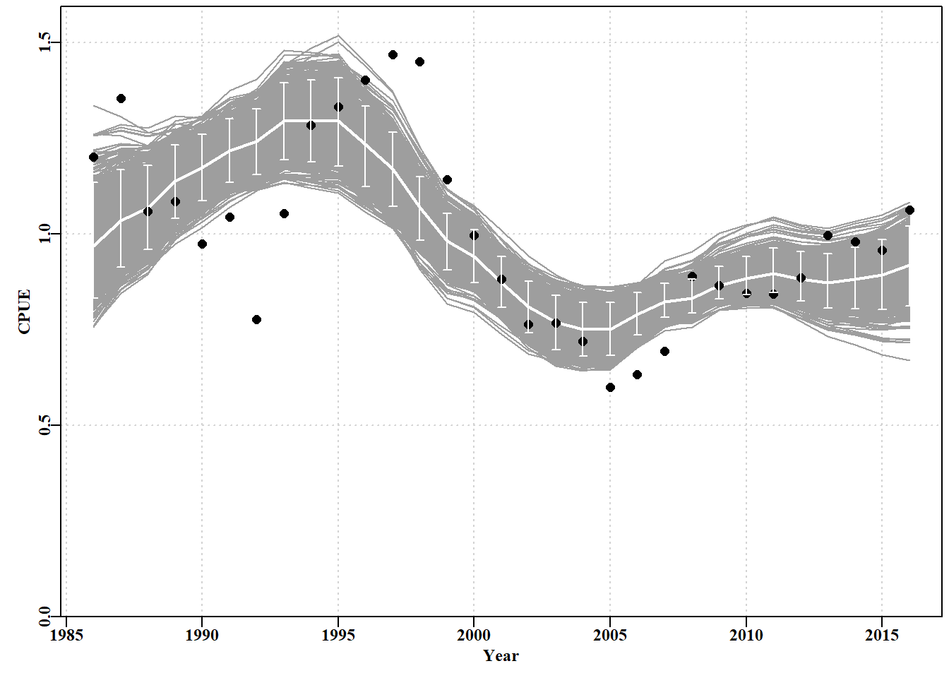
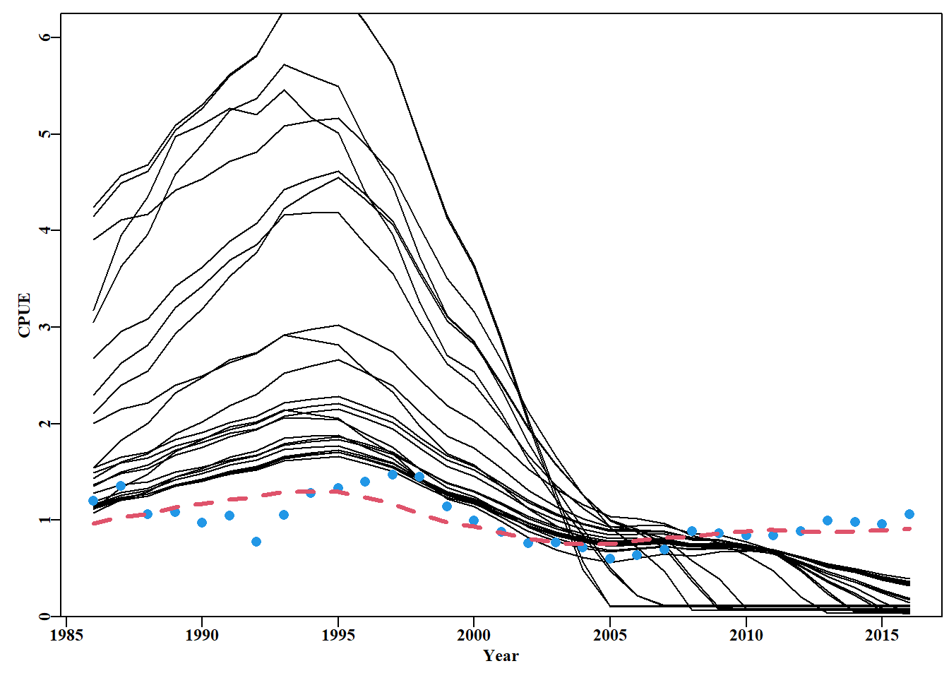
#data and trajectories from 1000 MVN parameter vectors Fig 7.16 plot1(fish[,"year"],fish[,"cpue"],type="p",xlab="Year",ylab="CPUE", maxy=2.0)for(iin1:N)lines(fish[,"year"],mvncpue[i,],col="grey",lwd=1)points(fish[,"year"],fish[,"cpue"],pch=1,cex=1.3,col=1,lwd=2)# data lines(fish[,"year"],exp(simpspm(optpar,fish)),lwd=2,col=1)# pred percs<-apply(mvncpue,2,quants)# obtain the quantiles arrows(x0=fish[,"year"],y0=percs["5%",],y1=percs["95%",],length=0.03, angle=90,code=3,col=1)#add 90% quantiles msy<-mvnpar[,"r"]*mvnpar[,"K"]/4# 1000 MSY estimates text(2010,1.75,paste0("MSY ",round(mean(msy),3)),cex=1.25,font=7)
图 7.16: 从最优参数及其相关方差-协方差矩阵定义的多变量正态分布中采样的随机参数向量得出的 1000 条 cpue 预测轨迹。The 1000 predicted cpue trajectories derived from random parameter vectors sampled from the multi-variate normal distribution defined by the optimum parameters and their related variance-covariance matrix.
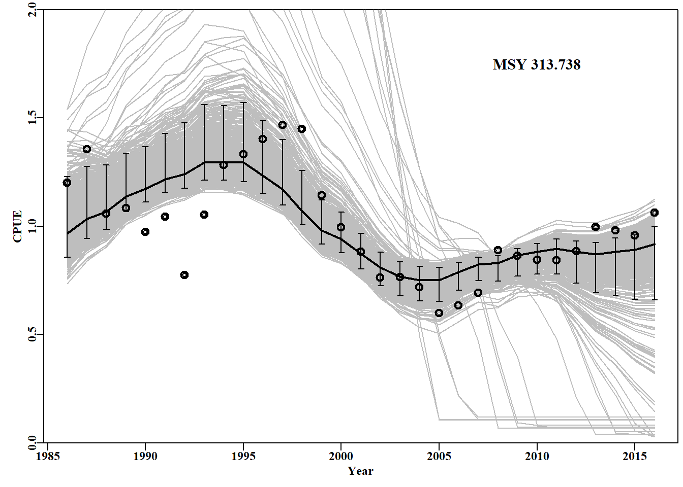
图 7.17: 预测 2016 年 cpue < 0.4 的 34 个渐近误差 cpue 轨迹。圆点为原始数据,虚线为最佳拟合模型。The 34 asymptotic error cpue trajectories that were predicted to have a cpue < 0.4 in 2016. The dots are the original data and the dashed line the optimum model fit.
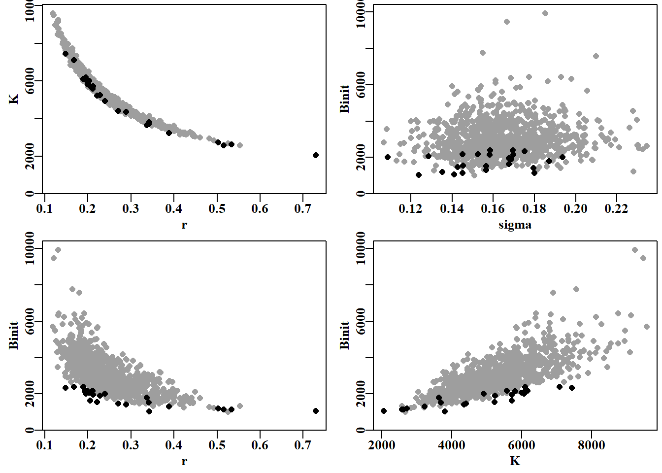
#Use adhoc function to plot errant parameters Fig 7.18 parset(plots=c(2,2),cex=0.85)outplot<-function(var1,var2,pickdev){plot1(mvnpar[,var1],mvnpar[,var2],type="p",pch=16,cex=1.0, defpar=FALSE,xlab=var1,ylab=var2,col=8)points(mvnpar[pickdev,var1],mvnpar[pickdev,var2],pch=16,cex=1.0)}outplot("r","K",pickd)# assumes mvnpar in working environment outplot("sigma","Binit",pickd)outplot("r","Binit",pickd)outplot("K","Binit",pickd)
图 7.18: 渐近误差样本中参数值的分布,黑色部分为预测最终 cpue < 0.4 的参数值。看来,Binit 的低值是造成难以置信轨迹的主要原因。The spread of parameter values from the asymptotic error samples with the values that predicted final cpue < 0.4 highlighted in black. It appears that low values of Binit are mostly behind the implausible trajectories.
图 7.19: 使用多变量正态分布生成参数组合时 Schaefer 模型参数之间的关系。r - K 之间的关系比自举样本紧密得多,而 sigma 与其他参数之间几乎没有关系。损耗图显示一些轨迹已经消失。The relationships between the model parameters for the Schaefer model when using the multi-variate normal distribution to generate the parameter combinations. The relationship between r - K is much tighter than in the bootstrap samples and there is almost no relationship between sigma and the other parameters. The depletion plots indicate some trajectories go extinct.
# Get the ranges of parameters from bootstrap and asymptotic bt<-apply(bootpar,2,range)[,c(1:4,6,7)]ay<-apply(mvnpar,2,range)out<-rbind(bt,ay)rownames(out)<-c("MinBoot","MaxBoot","MinAsym","MaxAsym")
表 7.7: 自举取样与渐近误差取样的参数值范围对比。The range of parameter values from the bootstrap sampling compared with those from the Asymptotic Error sampling.
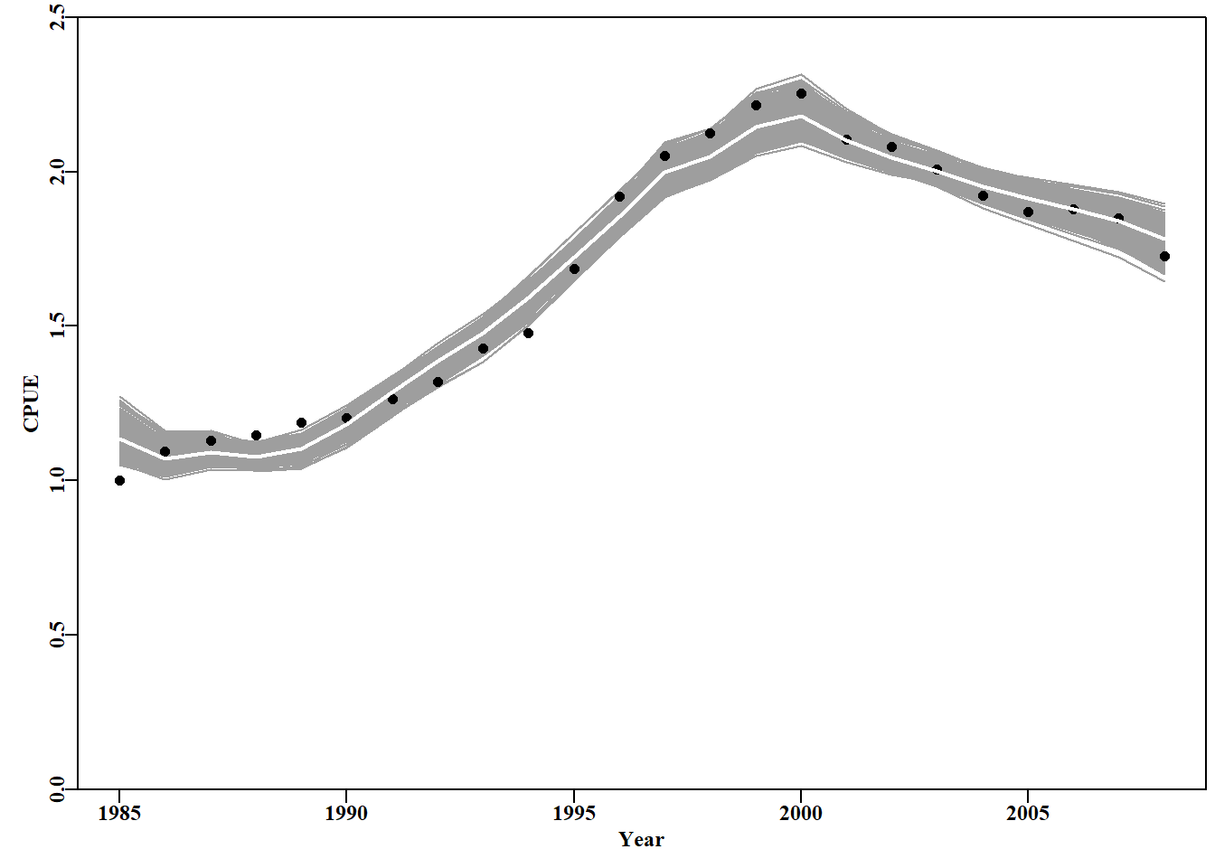
#repeat asymptotice errors using abdat data-set Figure 7.20 data(abdat)fish<-as.matrix(abdat)pars<-log(c(r=0.4,K=9400,Binit=3400,sigma=0.05))ansA<-fitSPM(pars,fish,schaefer=TRUE,maxiter=1000,hess=TRUE)vcovA<-solve(ansA$hessian)# calculate var-covar matrix mvn<-length(fish[,"year"])N<-1000# replicates mvncpueA<-matrix(0,nrow=N,ncol=mvn,dimnames=list(1:N,fish[,"year"]))columns<-c("r","K","Binit","sigma")optparA<-ansA$estimate# Fill matrix of parameter vectors mvnparA<-matrix(exp(rmvnorm(N,mean=optparA,sigma=vcovA)), nrow=N,ncol=4,dimnames=list(1:N,columns))msy<-mvnparA[,"r"]*mvnparA[,"K"]/4for(iin1:N)mvncpueA[i,]<-exp(simpspm(log(mvnparA[i,]),fish))mvnparA<-cbind(mvnparA,msy)plot1(fish[,"year"],fish[,"cpue"],type="p",xlab="Year",ylab="CPUE", maxy=2.5)for(iin1:N)lines(fish[,"year"],mvncpueA[i,],col=8,lwd=1)points(fish[,"year"],fish[,"cpue"],pch=16,cex=1.0)#orig data lines(fish[,"year"],exp(simpspm(optparA,fish)),lwd=2,col=0)
图 7.20: 利用渐近误差为 abdat 数据集生成可信的参数集及其隐含的 cpue 轨迹。最佳拟合模型以白线表示。The use of asymptotic errors to generate plausible parameter sets and their implied cpue trajectories for the abdat data-set. The optimum model fit is shown as a white line.
图 7.21: 将 Schaefer 模型拟合到 abdat 数据并使用多变量正态分布生成后续参数组合时的模型参数关系。这与 “不确定性”一章中的自举法非常相似。Model parameter relationships when fitting the Schaefer model to the abdat data and using the multi-variate normal distribution to generate subsequent parameter combinations. These are very similar to the bootstrap equivalent in the On Uncertainty chapter.
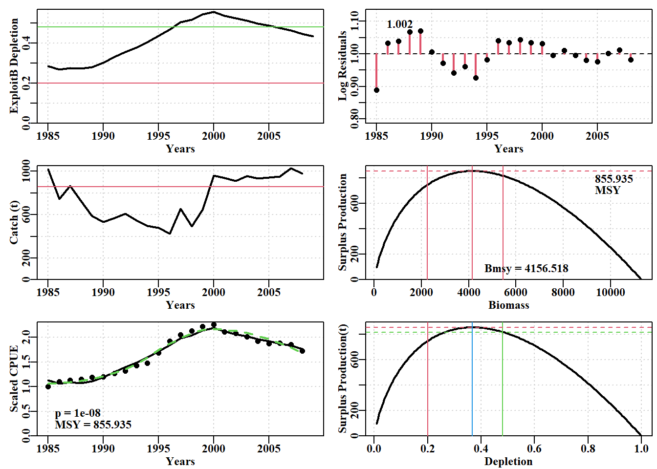
#Fit the Fox Model to the abdat data Figure 7.22 data(abdat); fish<-as.matrix(abdat)param<-log(c(r=0.3,K=11500,Binit=3300,sigma=0.05))foxmod<-nlm(f=negLL1,p=param,funk=simpspm,indat=fish, logobs=log(fish[,"cpue"]),iterlim=1000,schaefer=FALSE)optpar<-exp(foxmod$estimate)ans<-plotspmmod(inp=foxmod$estimate,indat=fish,schaefer=FALSE, addrmse=TRUE, plotprod=TRUE)
图 7.22: 使用 Fox 模型和对数正态误差拟合的 abdat 数据集最佳模型。绿色虚线是较平滑的曲线,红线是最佳预测模型拟合。请注意对数正态残差的模式,这表明该模型在该数据方面存在微小不足。The optimum model fit for the abdat data-set using the Fox model and log-normal errors. The green dashed line is a smoother curve while the red line is the optimum predicted model fit. Note the pattern in the log-normal residuals indicating that the model has small inadequacies with regard to this data.
#|echo: falselibrary(Rcpp)cppFunction('NumericVector simpspmC(NumericVector pars, NumericMatrix indat, LogicalVector schaefer) { int nyrs = indat.nrow(); NumericVector predce(nyrs); NumericVector biom(nyrs+1); double Bt, qval; double sumq = 0.0; double p = 0.00000001; if (schaefer(0) == TRUE) { p = 1.0; } NumericVector ep = exp(pars); biom[0] = ep[2]; for (int i = 0; i < nyrs; i++) { Bt = biom[i]; biom[(i+1)] = Bt + (ep[0]/p)*Bt*(1 - pow((Bt/ep[1]),p)) - indat(i,1); if (biom[(i+1)] < 40.0) biom[(i+1)] = 40.0; sumq += log(indat(i,2)/biom[i]); } qval = exp(sumq/nyrs); for (int i = 0; i < nyrs; i++) { predce[i] = log(biom[i] * qval); } return predce; }')
代码
# eval: false# Conduct an MCMC using simpspmC on the abdat Fox SPM # This means you will need to compile simpspmC from appendix set.seed(698381)#for repeatability, possibly only on Windows10 begin<-gettime()# to enable the time taken to be calculated inscale<-c(0.07,0.05,0.09,0.45)#note large value for sigma pars<-log(c(r=0.205,K=11300,Binit=3200,sigma=0.044))result<-do_MCMC(chains=1,burnin=50,N=2000,thinstep=512, inpar=pars,infunk=negLL,calcpred=simpspm, obsdat=log(fish[,"cpue"]),calcdat=fish, priorcalc=calcprior,scales=inscale,schaefer=FALSE)# alternatively, use simpspm, but that will take longer. cat("acceptance rate = ",result$arate," \n")
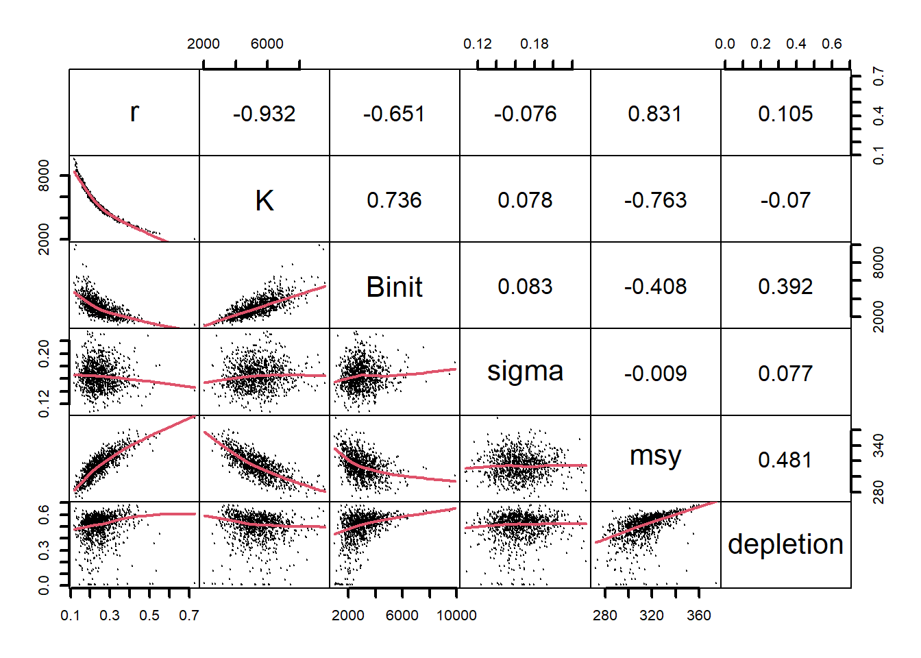
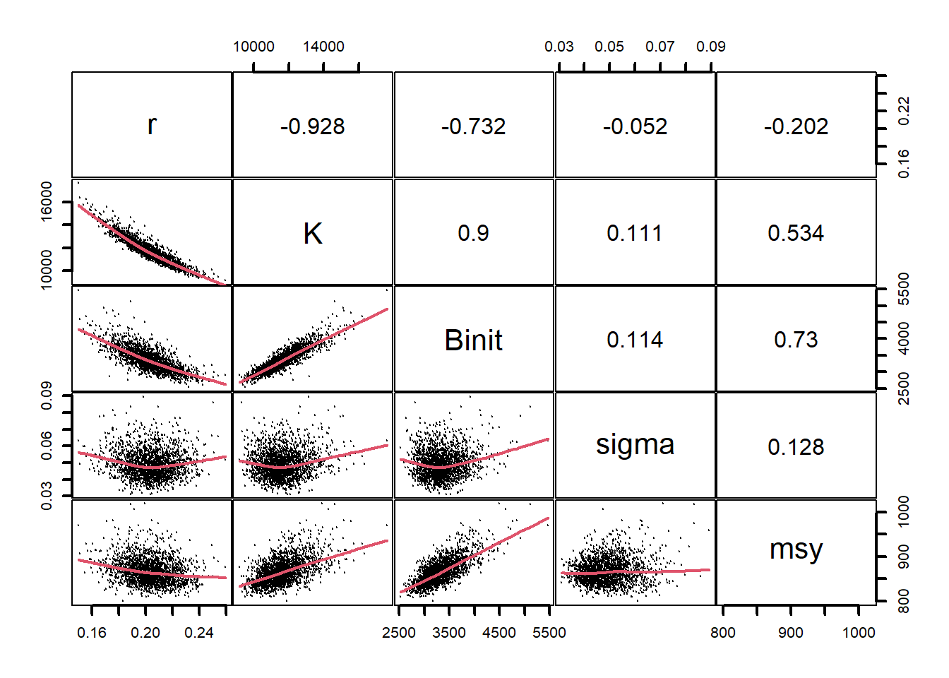
#pairwise comparison for MCMC of Fox model on abdat Fig 7.23 pairs(cbind(post1[,1:4],msy),upper.panel =panel.cor,lwd=2,cex=0.2, lower.panel=panel.smooth,col=1,gap=0.1)
图 7.23: MCMC 输出的成对散点图。实线是表示趋势的塬平滑线,上半部分的数字是成对散点图之间的相关系数。r、K 和 Binit 之间,以及 K、Binit 和 MSY 之间都有很强的相关性,而 sigma 与其他参数或 msy 与 r 之间的关系较小或没有关系。MCMC output as paired scattergrams. The solid lines are loess smoothers indicating trends and the numbers in the upper half are the correlation coefficients between the pairs. Strong correlations are indicated between r, K, and Binit, and between K, Binit, and MSY, with only minor or no relationships between sigma the other parameters or between msy and r.
代码
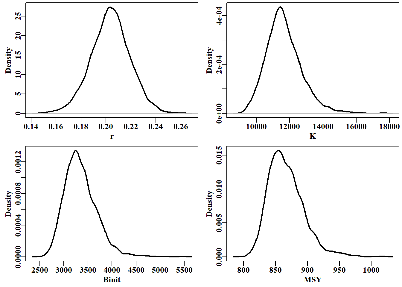
# marginal distributions of 3 parameters and msy Figure 7.24 parset(plots=c(2,2), cex=0.85)plot(density(post1[,"r"]),lwd=2,main="",xlab="r")#plot has a method plot(density(post1[,"K"]),lwd=2,main="",xlab="K")#for output from plot(density(post1[,"Binit"]),lwd=2,main="",xlab="Binit")# density plot(density(msy),lwd=2,main="",xlab="MSY")#try str(density(msy))
图 7.24: 将 Fox 模型应用于鳕鱼数据的 2000 次 MCMC 重复计算得出的三个参数的边际分布和隐含的 MSY。曲线的块状表明需要进行 2000 次以上的迭代。The marginal distributions for three parameters and the implied MSY from 2000 MCMC replicates for the Fox model applied to the abdat data. The lumpiness of the curves suggests more than 2000 iterations are needed.
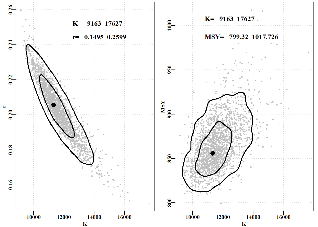
#MCMC r and K parameters, approx 50 + 90% contours. Fig7.25 puttxt<-function(xs,xvar,ys,yvar,lvar,lab="",sigd=0){text(xs*xvar[2],ys*yvar[2],makelabel(lab,lvar,sep=" ", sigdig=sigd),cex=1.2,font=7,pos=4)}# end of puttxt - a quick utility function kran<-range(post1[,"K"]); rran<-range(post1[,"r"])mran<-range(msy)#ranges used in the plots parset(plots=c(1,2),margin=c(0.35,0.35,0.05,0.1))#plot r vs K plot(post1[,"K"],post1[,"r"],type="p",cex=0.5,xlim=kran, ylim=rran,col="grey",xlab="K",ylab="r",panel.first=grid())points(optpar[2],optpar[1],pch=16,col=1,cex=1.75)# center addcontours(post1[,"K"],post1[,"r"],kran,rran, #if fails make contval=c(0.5,0.9),lwd=2,col=1)#contval smaller puttxt(0.7,kran,0.97,rran,kran,"K= ",sigd=0)puttxt(0.7,kran,0.94,rran,rran,"r= ",sigd=4)plot(post1[,"K"],msy,type="p",cex=0.5,xlim=kran, # K vs msy ylim=mran,col="grey",xlab="K",ylab="MSY",panel.first=grid())points(optpar[2],getMSY(optpar,p),pch=16,col=1,cex=1.75)#center addcontours(post1[,"K"],msy,kran,mran,contval=c(0.5,0.9),lwd=2,col=1)puttxt(0.6,kran,0.99,mran,kran,"K= ",sigd=0)puttxt(0.6,kran,0.97,mran,mran,"MSY= ",sigd=3)
图 7.25: MCMC 边际分布输出为 r 和 K 参数以及 K 和 MSY 值的散点图。灰点是成功的候选参数向量,等值线是近似的第 50 和第 90 分位数。文中给出了全部可接受的参数迹线范围。MCMC marginal distributions output as a scattergram of the r and K parameters, and the K and MSY values. The grey dots are from successful candidate parameter vectors, while the contours are approximate 50th and 90th percentiles. The text give the full range of the accepted parameter traces.
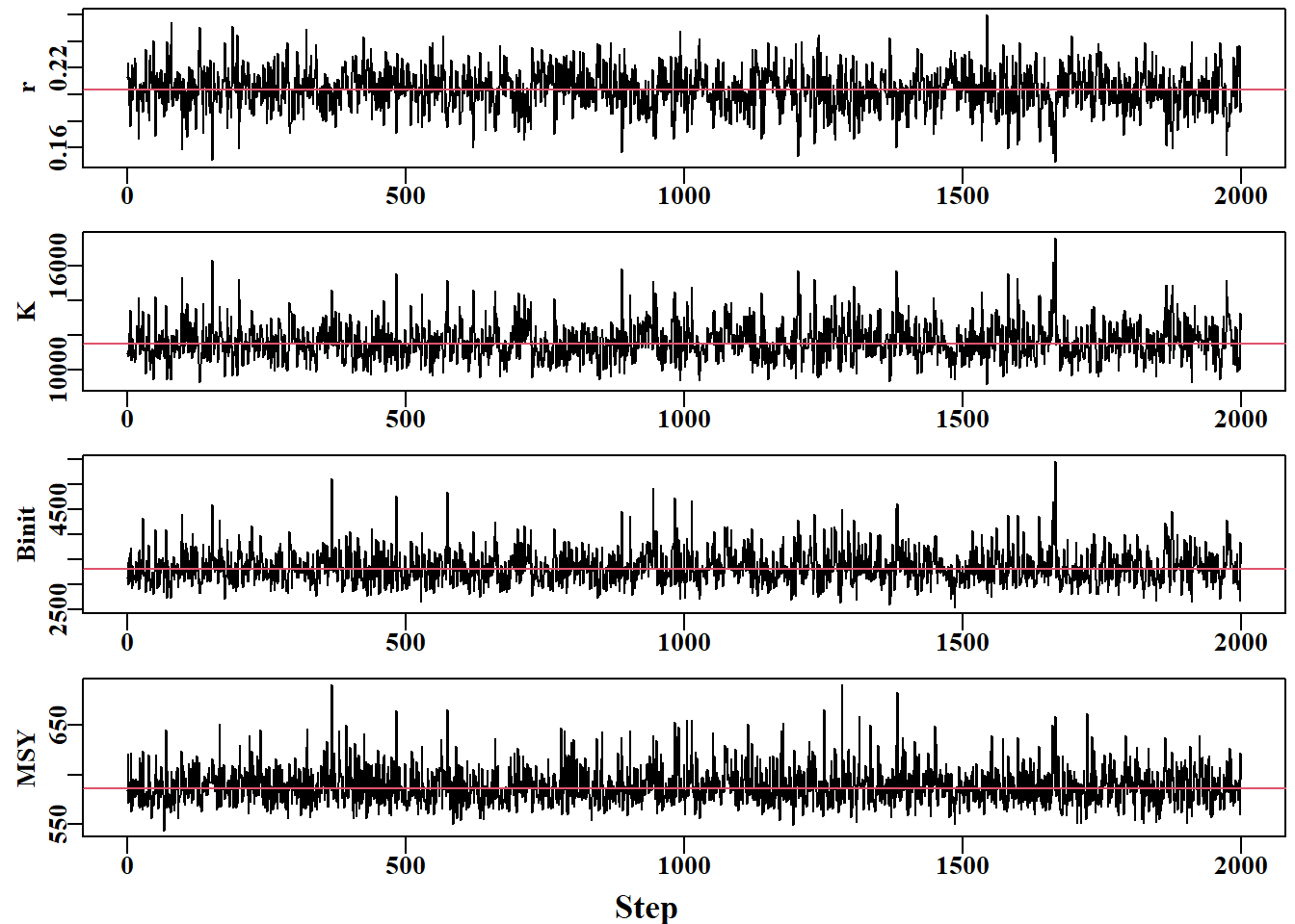
#Traces for the Fox model parameters from the MCMC Fig7.26 parset(plots=c(4,1),margin=c(0.3,0.45,0.05,0.05), outmargin =c(1,0,0,0),cex=0.85)label<-colnames(post1)N<-dim(post1)[1]for(iin1:3){plot(1:N,post1[,i],type="l",lwd=1,ylab=label[i],xlab="")abline(h=median(post1[,i]),col=2)}msy<-post1[,1]*post1[,2]/4plot(1:N,msy,type="l",lwd=1,ylab="MSY",xlab="")abline(h=median(msy),col=2)mtext("Step",side=1,outer=T,line=0.0,font=7,cex=1.1)
三个主要 Schaefer 模型参数和 MSY 估计值的迹线。如果细化步长增加到 1024 步或更长,迹线内剩余的自相关性应得到改善。The traces for the three main Schaefer model parameters and the MSY estimates. The remaining auto-correlation within traces should be improved if the thinning step were increased to 1024 or longer.
#Do five chains of the same length for the Fox model set.seed(6396679)# Note all chains start from same place, which is inscale<-c(0.07,0.05,0.09,0.45)# suboptimal, but still the chains pars<-log(c(r=0.205,K=11300,Binit=3220,sigma=0.044))# differ result<-do_MCMC(chains=5,burnin=50,N=2000,thinstep=512, inpar=pars,infunk=negLL1,calcpred=simpspmC, obsdat=log(fish[,"cpue"]),calcdat=fish, priorcalc=calcprior,scales=inscale, schaefer=FALSE)cat("acceptance rate = ",result$arate," \n")# always check this
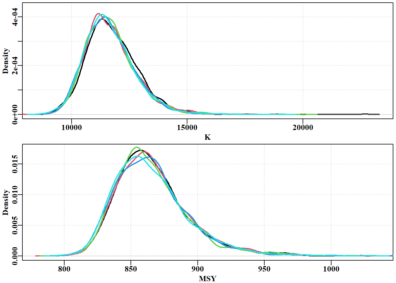
#Now plot marginal posteriors from 5 Fox model chains Fig7.27 parset(plots=c(2,1),cex=0.85,margin=c(0.4,0.4,0.05,0.05))post<-result[[1]][[1]]plot(density(post[,"K"]),lwd=2,col=1,main="",xlab="K", ylim=c(0,4.4e-04),panel.first=grid())for(iin2:5)lines(density(result$result[[i]][,"K"]),lwd=2,col=i)p<-1e-08post<-result$result[[1]]msy<-post[,"r"]*post[,"K"]/((p+1)^((p+1)/p))plot(density(msy),lwd=2,col=1,main="",xlab="MSY",type="l", ylim=c(0,0.0175),panel.first=grid())for(iin2:5){post<-result$result[[i]]msy<-post[,"r"]*post[,"K"]/((p+1)^((p+1)/p))lines(density(msy),lwd=2,col=i)}
图 7.26: K 参数的边际后验值和 5 链 2000 次重复(512 * 2000 = 1049600 次迭代)得出的隐含 MSY。分布之间仍存在一些差异,尤其是在模式处,这表明更多的重复和更高的稀疏率可能会改善结果。the marginal posterior for the K parameter and the implied MSY from five chains of 2000 replicates (512 * 2000 = 1049600 iterations). Some variation remains between the distributions, especially at the mode, suggesting that more replicates and potentially a higher thinning rate would improve the outcome.
# get qunatiles of each chain probs<-c(0.025,0.05,0.5,0.95,0.975)storeQ<-matrix(0,nrow=6,ncol=5,dimnames=list(1:6,probs))for(iin1:5)storeQ[i,]<-quants(result$result[[i]][,"K"])x<-apply(storeQ[1:5,],2,range)storeQ[6,]<-100*(x[2,]-x[1,])/x[2,]
表 7.8: 针对 abdat 数据的 Fox 模型运行的五条 MCMC 链中 K 参数的五个量化值。最后一行是各链数值范围的百分比差异,显示它们的中位数相差略高于 1%。Five quantiles on the K parameter from the five MCMC chains run on the Fox model applied to the abdat data. The last row is the percent difference in the range of the values across the chains, which shows their medians differ by slightly more than 1%.
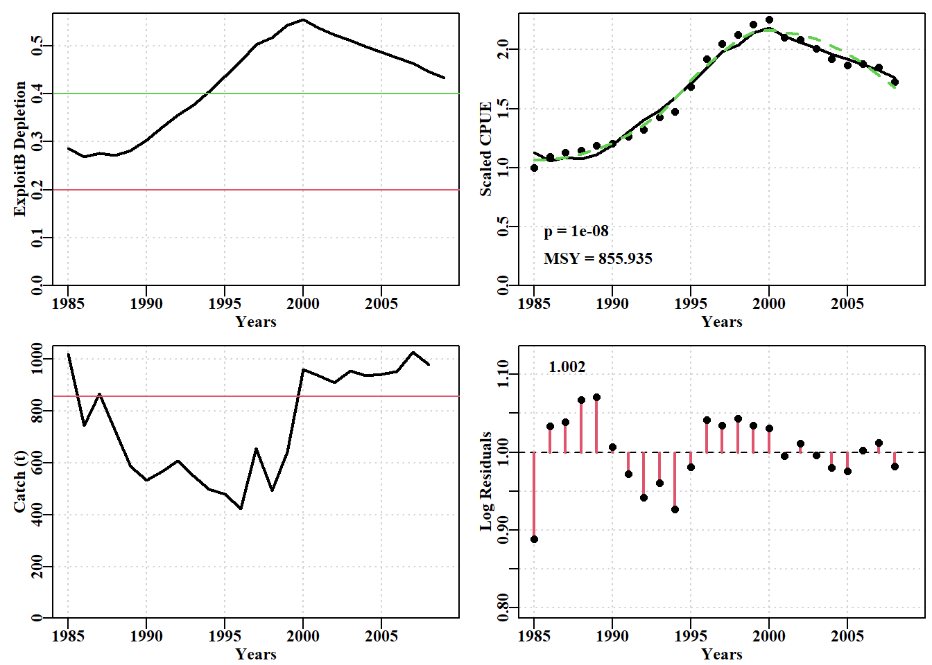
#Prepare Fox model on abdat data for future projections Fig7.28 data(abdat); fish<-as.matrix(abdat)param<-log(c(r=0.3,K=11500,Binit=3300,sigma=0.05))bestmod<-nlm(f=negLL1,p=param,funk=simpspm,schaefer=FALSE, logobs=log(fish[,"cpue"]),indat=fish,hessian=TRUE)optpar<-exp(bestmod$estimate)ans<-plotspmmod(inp=bestmod$estimate,indat=fish,schaefer=FALSE, target=0.4,addrmse=TRUE, plotprod=FALSE)
图 7.27: 使用 Fox 模型和对数正态误差拟合的 abdat 数据集最佳模型。绿色虚线为黄土曲线,红色实线为最佳预测拟合模型。请注意对数正态残差的模式,这表明该模型在该数据方面存在一些不足。The optimum model fit for the abdat data-set using the Fox model and log-normal errors. The green dashed line is a loess curve while the solid red line is the optimum predicted model fit. Note the pattern in the log-normal residuals indicating that the model has some inadequacies with regard to this data.
表 7.9: 前十行为 abdat 数据集所代表的种群动态预测值和最佳 Fox 模型拟合值。The first ten rows of the predicted dynamics of the stock represented by the abdat data-set and the optimal Fox model fit.
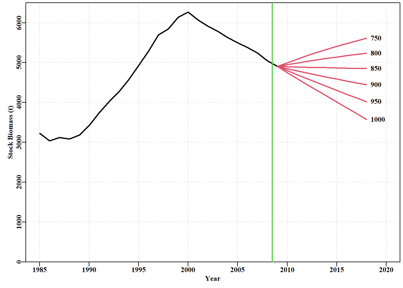
# Fig 7.29 catches<-seq(700,1000,50)# projyr=10 is the default projans<-spmprojDet(spmobj=out,projcatch=catches,plotout=TRUE)
图 7.28: 根据 abdat 数据集拟合的最佳 Fox 模型的确定性恒定渔获量预测。垂直绿线是可用数据的极限,其右侧的红线是主要预测。数字是施加的恒定渔获量。Deterministic constant catch projections of the optimum Fox model fit to the abdat data-set. the vertical green line is the limit of the data available and the red lines to the right of that are the main projections. The numbers are the constant catches imposed.
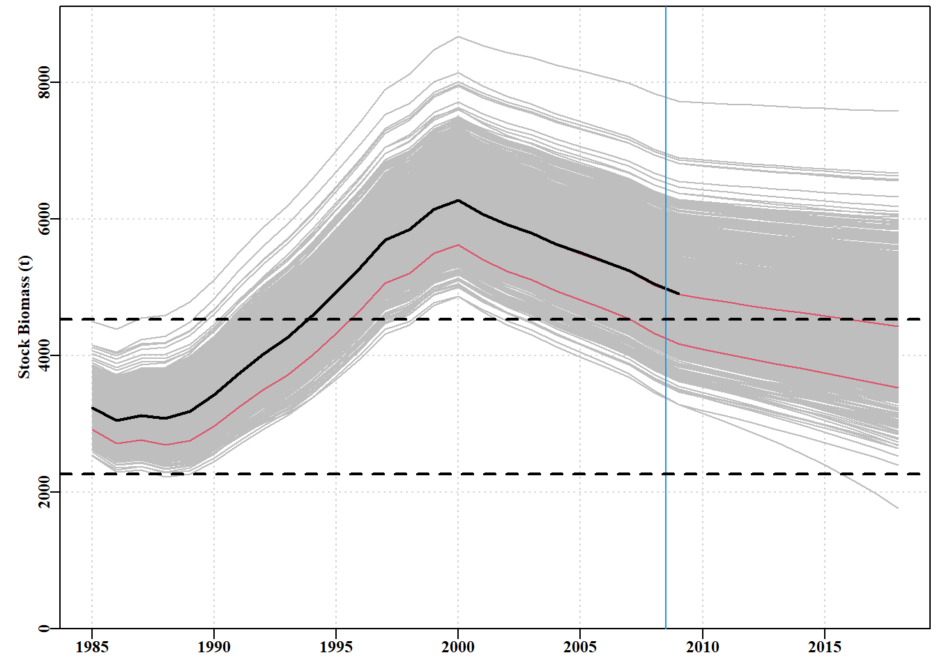
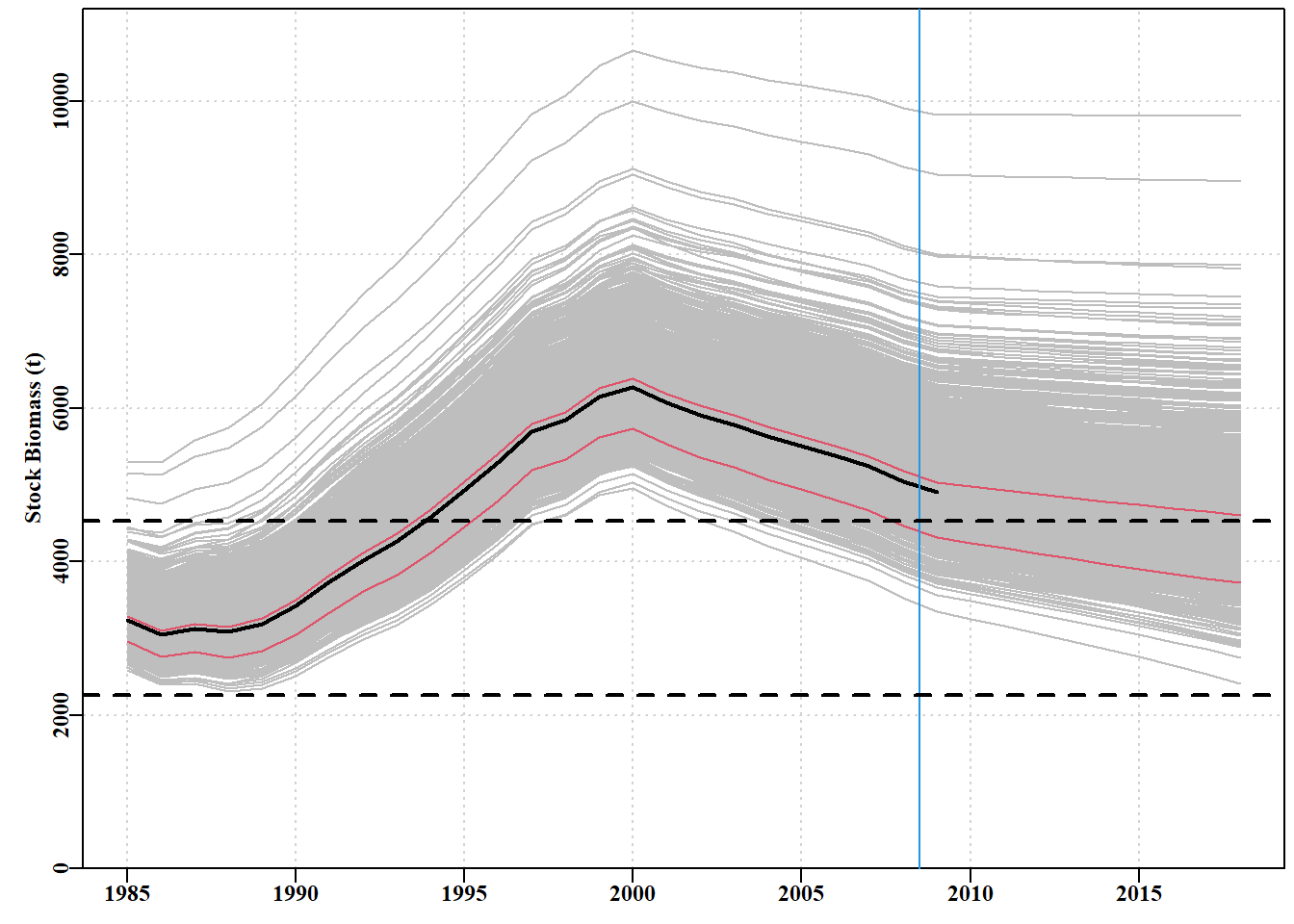
# generate parameter vectors from a multivariate normal # project dynamics under a constant catch of 900t library(mvtnorm)matpar<-parasympt(bestmod,N=1000)#generate parameter vectors projs<-spmproj(matpar,fish,projyr=10,constC=900)#do dynamics
图 7.29: 1000 个预测值,通过使用反向哈希值和平均参数估计值生成 1000 个可信参数向量,并将每 个向量与 10 年不变的 900 吨渔获量后的渔获量向前推算得出。虚线为极限和目标参考点。蓝色垂直线是渔业数据的极限,黑色粗线是最优拟合,与最优线平行的红色细线是各年的第 10 和第 50 个量值。1000 projections derived from the using the inverse hessian and mean parameter estimates to generate 1000 plausible parameter vectors and projecting each vector forward with the fisheries catches followed by 10 years of a constant catch of 900t. The dashed lines are the limit and target reference points. The blue vertical line is the limit of fisheries data, the thick black line is the optimum fit and the thin red lines parallel to the optimum line are the 10th and 50th quantiles across years.
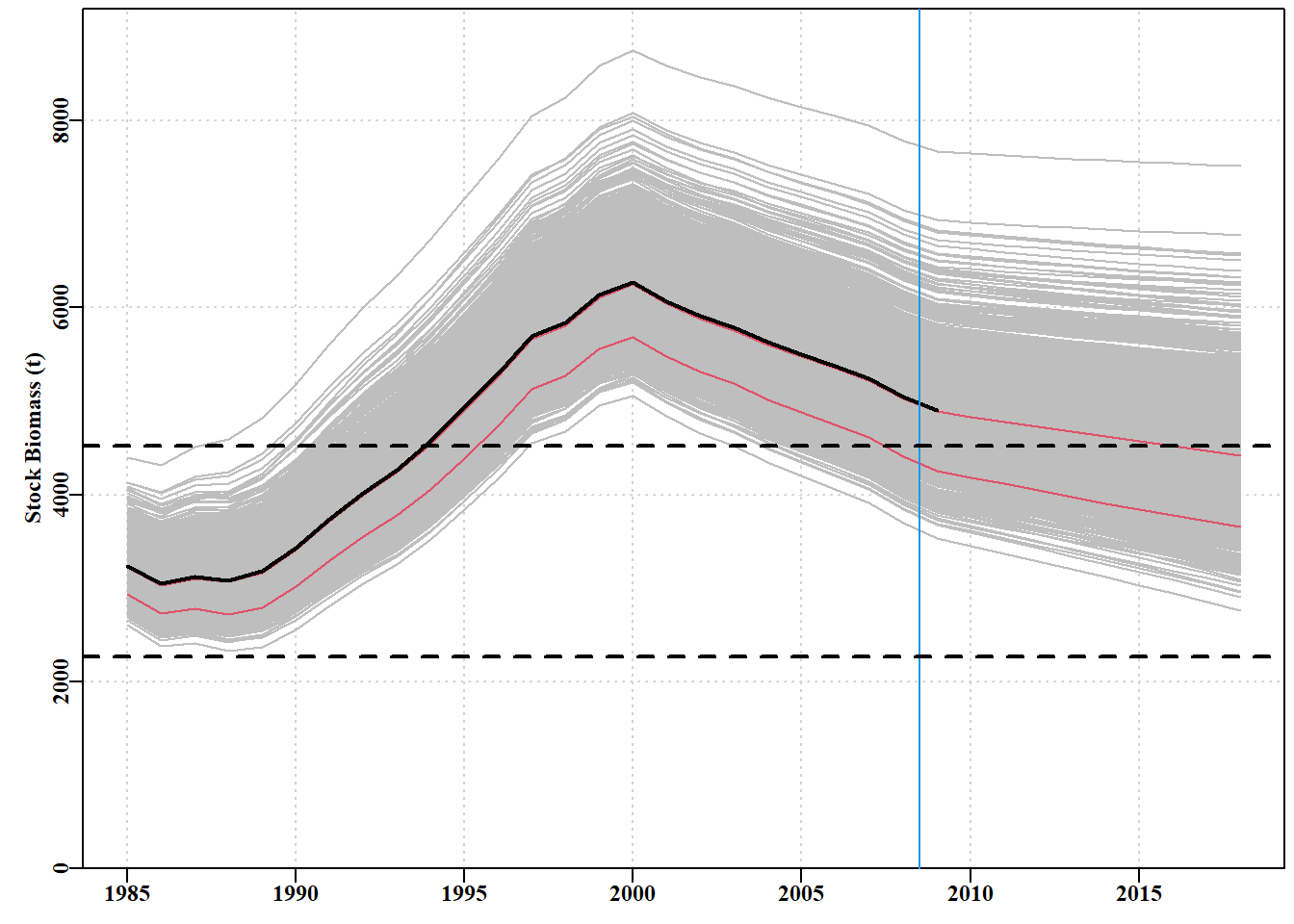
#bootstrap generation of plausible parameter vectors for Fox reps<-1000boots<-spmboot(bestmod$estimate,fishery=fish,iter=reps, schaefer=FALSE)matparb<-boots$bootpar[,1:4]#examine using head(matparb,20)
#bootstrap projections. Lower case b for boostrap Fig7.31 projb<-spmproj(matparb,fish,projyr=10,constC=900)outb<-plotproj(projb,out,qprob=c(0.1,0.5),refpts=c(0.2,0.4))
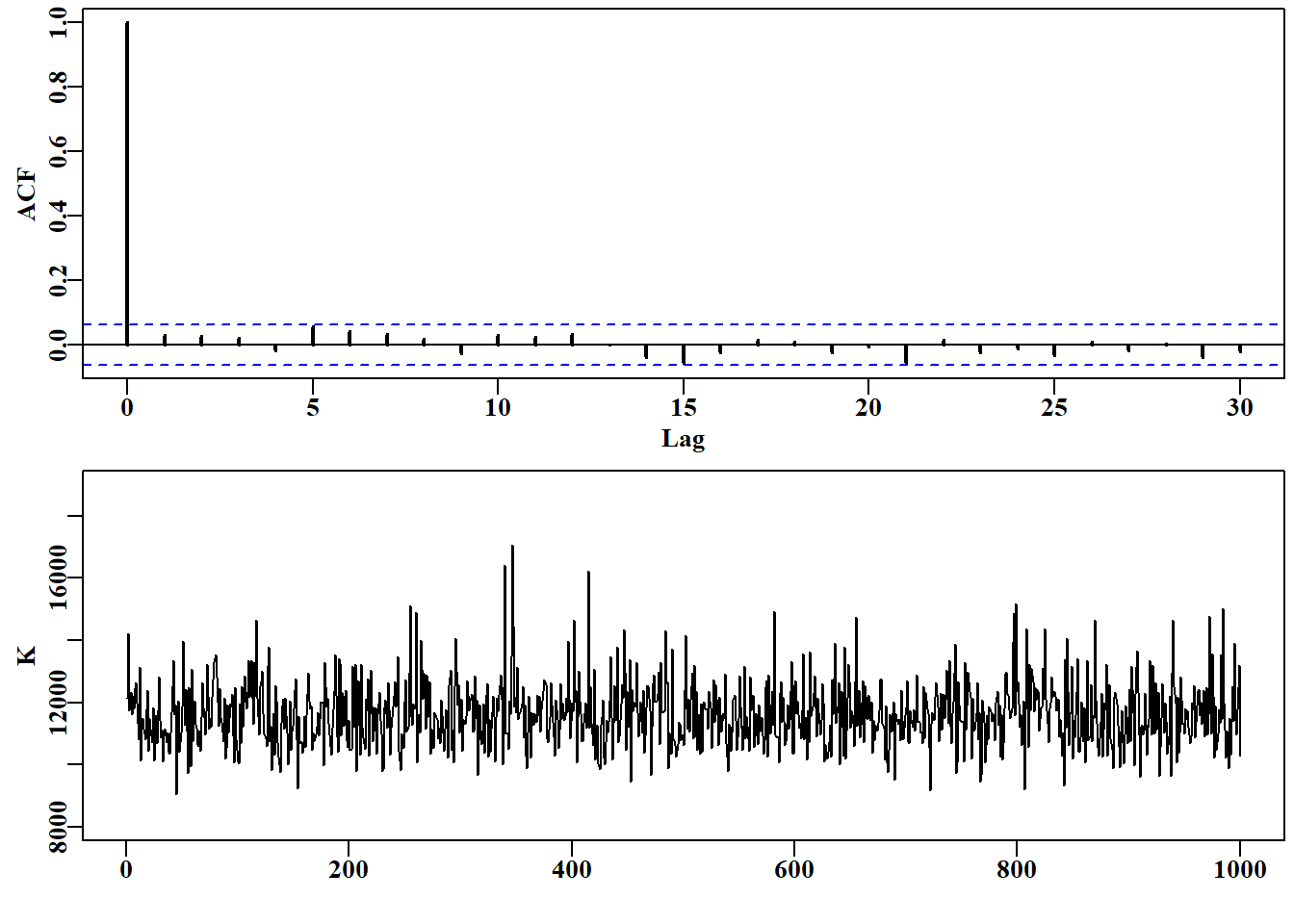
# auto-correlation, or lack of, and the K trace Fig 7.32 parset(plots=c(2,1),cex=0.85)acf(parB[,2],lwd=2)plot(1:N,parB[,2],type="l",ylab="K",ylim=c(8000,19000),xlab="")
图 7.31: 从上图可以明显看出,过剩产量模型福克斯版本的 K 参数后验分布的 1000 次抽样中缺乏自相关性。下图中的迹线显示了典型的分散值,但保留了一些更极端的峰值。
# Fig 7.33 matparB<-as.matrix(parB[,1:4])# B for Bayesian projs<-spmproj(matparB,fish,constC=900,projyr=10)# project them plotproj(projs,out,qprob=c(0.1,0.5),refpts=c(0.2,0.4))#projections
在贝叶斯分析中,我们希望使用 Fox 剩余产量模型。这当然可以使用函数 simpspm(),通过修改 schaefer 参数来实现。但是
代码
library(Rcpp)cppFunction('NumericVector simpspmC(NumericVector pars, NumericMatrix indat, LogicalVector schaefer) { int nyrs = indat.nrow(); NumericVector predce(nyrs); NumericVector biom(nyrs+1); double Bt, qval; double sumq = 0.0; double p = 0.00000001; if (schaefer(0) == TRUE) { p = 1.0; } NumericVector ep = exp(pars); biom[0] = ep[2]; for (int i = 0; i < nyrs; i++) { Bt = biom[i]; biom[(i+1)] = Bt + (ep[0]/p)*Bt*(1 - pow((Bt/ep[1]),p)) - indat(i,1); if (biom[(i+1)] < 40.0) biom[(i+1)] = 40.0; sumq += log(indat(i,2)/biom[i]); } qval = exp(sumq/nyrs); for (int i = 0; i < nyrs; i++) { predce[i] = log(biom[i] * qval); } return predce; }')
Elder, R. D. 1979. 《Equilibrium Yield for the Hauraki Gulf Snapper Fishery Estimated from Catch and Effort Figures, 196074》. New Zealand Journal of Marine and Freshwater Research 13 (1): 31–38. https://doi.org/10.1080/00288330.1979.9515778.
Hilborn, Ray. 1979. 《Comparison of Fisheries Control Systems That Utilize Catch and Effort Data》. Journal of the Fisheries Research Board of Canada 36 (12): 1477–89. https://doi.org/10.1139/f79-215.
MacCall, Alec D. 2009. 《Depletion-Corrected Average Catch: A Simple Formula for Estimating Sustainable Yields in Data-Poor Situations》. ICES Journal of Marine Science 66 (10): 2267–71. https://doi.org/10.1093/icesjms/fsp209.
Polacheck, Tom, Ray Hilborn, 和 Andre E. Punt. 1993. 《Fitting Surplus Production Models: Comparing Methods and Measuring Uncertainty》. Canadian Journal of Fisheries and Aquatic Sciences 50 (12): 2597–607. https://doi.org/10.1139/f93-284.
Prager, Michael. 1994. 《A suite of extensions to a nonequilibrium surplus-production model》. Fishery Bulletin 92 (一月): 374–89.
Punt, Andre E., 和 Ray Hilborn. 1997. 《Fisheries Stock Assessment and Decision Analysis: The Bayesian Approach》. Reviews in Fish Biology and Fisheries 7 (1): 35–63. https://doi.org/10.1023/A:1018419207494.
Saila, S. B., J. H. Annala, J. L. McKoy, 和 J. D. Booth. 1979. 《Application of Yield Models to the New Zealand Rock Lobster Fishery》. New Zealand Journal of Marine and Freshwater Research 13 (1): 1–11. https://doi.org/10.1080/00288330.1979.9515775.
Schaefer, M. 1991. 《Some Aspects of the Dynamics of Populations Important to the Management of the Commercial Marine Fisheries》. Bulletin of Mathematical Biology 53 (1-2): 253–79. https://doi.org/10.1016/s0092-8240(05)80049-7.
Winker, Henning, Felipe Carvalho, 和 Maia Kapur. 2018. 《JABBA: Just Another Bayesian Biomass Assessment》. Fisheries Research 204 (八月): 275–88. https://doi.org/10.1016/j.fishres.2018.03.010.
源代码
# 剩余产量模型 {#sec-surplusproduction}## 引言在前面的章节中,我们已经使用并拟合了所谓的静态模型,这些模型在一段时间内是稳定的(*例如*,使用`vB()` 、`Gz()`或`mm()` 的生长模型 )。此外,在第 [-@sec-paraestimat] 章 [模型参数估计](04-application.qmd) 和第 [-@sec-uncertainty] 章[不确定性](06-uncertainty.qmd)两章中,我们已经介绍了剩余产量模型(surplus production model, spm),这些模型可用于进行资源评估(例如 Schaefer 模型),并提供了一个时间序列数据的动态模型的示例。然而,当我们专注于特定的建模方法时,此类模型的细节开发受到限制。我们将在本章深入研究剩余产量模型。剩余产量模型(或者生物量动态模型)[@hilborn1992] 将补充、生长和死亡率(生产的所有方面)的总体效应汇集到一个单一的生产方程中,处理无差异的生物量(或数量)。“无差异的(undifferentiated)”一词意味着忽略了年龄和长度组成以及性别和其他差异的所有方面,实际上都被忽略了。为了进行正式的种群评估,就必须以某种方式对已开发资源的动态行为和生产力进行建模。这些动态的主要组分是种群对不同捕捞压力随时间推移的反应方式,即其资源量增加或减少的程度。通过研究不同捕捞强度水平的影响,一般可以评估种群的生产力。剩余产量模型提供了最简单的种群评估,尝试在模型与渔业数据拟合的基础上对种群动态进行描述。在20世纪50年代,@schaefer1957; @schaefer1991 描述了如何使用剩余产量模型来生成渔业种群评估。此后,这些模型得到很多发展 [@hilborn1992; @prager1994; @haddon2011; @winker2018],我们将在本章简要介绍这些较近期的动态模型。### 数据需求估算这种模型的现代离散模型参数所需的最基本数据至少是一个相对丰度指数的时间序列和一个相关的渔获量数据时间序列。渔获量数据可以涵盖比相对丰度指数数据的年份更长。简单模型中使用的相对种群丰度指数一般是单位努力渔获量(cpue),但也可以是一些与渔业无关的丰度指数(例如,来自拖网调查、声学调查),或者两者皆具。### 对比的需求尽管最近偶尔使用 [@elder1979; @saila1979; @punt1997],但剩余产量模型在 20 世纪 80 年代似乎不再流行。可能是因为在开发这些模型的早期,须假设被评估的种群处于平衡状态 [@elder1979; @saila1979],而这往往导致过于乐观的结论,从长远来看是站不住脚的。@hilborn1979 分析了许多此类情况,并证明使用的数据往往过于单一;他们的努力量水平上缺乏对比,因此对相关种群的动态缺乏信息。数据缺乏对比度意味着渔获量和努力量信息只能用于有限范围的种群丰度水平和有限的捕捞强度水平。有限的努力强度范围意味着对不同捕捞强度水平的反应范围也将有限。当种群动态更多地受环境因素而非渔获量的驱动时,也会出现这种对比的缺乏,因此种群似乎以意想不到的方式对渔业做出反应(例如,尽管渔获量或努力量没有变化,但种群发生了巨大变化)。剩余产量模型的一个重要假设是,所使用的相对丰度度量能够提供了种群相对丰度随时间的信息指标。一般来说,假设种群丰度与 CPUE 或其他指数之间存在线性关系(尽管这不一定是 1:1 的关系)。显而易见的风险是,这个假设要么是错误的,要么可以根据情况发生变化。例如,cpue 可能会变得非常稳定,这意味着即使种群数量减少或增加,它也不会发生变化。或者,由于外部因素影响,指数的变化可能会非常大,以至于无法检测到丰度趋势。例如,可能会观察到不同年份间 CPUE 的巨大变化,但考虑到种群的生产力,这种变化在生物学上是不可能的 (Haddon,2018)。一个不同但相关的假设是,努力量的质量和随后的渔获率在一段时间内保持不变。不幸的是,由于捕捞网具的技术变化、捕捞行为或方法的改变,或捕捞效率的其他变化,从而形成“努力量爬升”的概念,对于依赖 CPUE 作为相对丰度指数的评估来说,总是一个挑战或问题。努力量递增变的概念意味着努力量的有效性增加,因此任何基于名义努力量观测到的名义 cpue都会高估相对种群丰度(偏高)。cpue 的统计标准化 (Kimura,1981;Haddon,2018)可以解决其中一些问题,但显然只能考虑可获得数据的因素。例如,如果在渔业中引入 GPS 绘图仪或彩色回声测深仪,这往往会提高捕捞效率,但却没有记录哪些船只以及何时引入这些设备,那么这些设备对渔获率的正面影响将无法通过标准化来解释。### 渔获率何时具有参考价值检验丰度与任何相对丰度指数之间的假定关系是否真实和有信息的一个可能方法是,在发达渔业中,如果允许渔获量增加,预计 cpue 会在一段时间后开始下降。同样,如果渔获量减少到小于剩余产量(可能是通过管理或营销变化),那么随着种群规模的增加,预计cpue会在一段时间后很快增加。其原理是,如果渔获量低于种群当前的产量,那么最终种群规模和 cpue 都会增加,反之亦然。如果渔获量因供应不足而下降,但仍保持或高于当前生产力,则 cpue 当然不会增加,甚至可能进一步下降,尽管渔获量可能略有减少。重点放在发达渔业上,因为当渔业开始时,生物量的任何初始枯竭都会导致 “意外”渔 获量 [@maccall2009],因为种群被捕捞减少,这反过来又会导致 cpue 水平,一旦种群从未捕获水平减少,cpue 水平将无法维持。因此,预计在发达渔业中,cpue 在许多情况下与渔获量呈负相关,可能在 cpue 随渔获量变化而变化之间存在时滞。如果我们能发现这种关系,通常意味着数据中存在一定程度的反差;如果我们找不到这种负相关关系,通常意味着数据中有关种群如何对渔业做出反应的信息含量太低,无法仅根据渔获量和相对丰度指数进行评估。也就是说,在渔获量的基础上,相对丰度指数几乎没有增加更多的信息。我们将使用 **MQMF** 数据集 *schaef* 来说明这些观点。*Schaefer* 包含 @schaefer1957 原始黄鳍金枪鱼数据的渔获量和 CPUE,这是使用剩余产量模型进行种群评估的早期范例。```{r}#| label: tbl-spm1#| tbl-cap: |#| 1934 - 1955年的黄鳍金枪鱼渔业数据(Schaefer,1957)。#| 渔获量以千磅为单位,努力量以千个标准4级剪网日为单位,cpue以千磅/日为单位。 #| layout-ncol: 2# Yellowfin-tuna data from Schaefer 12957library(MQMF)library(tidyverse)library(gt)library(patchwork)library(knitr)data(schaef)kable(schaef[1:11,], digits =3, row.names =FALSE)kable(schaef[12:22,], digits =3, row.names =FALSE)```渔获量、cpue 及其关系图([@fig-spm1])仅显示 cpue 和渔获量之间微弱的负相关关系。如果我们用 `summary(model)` 检验 `lm()` 回归结果,我们发现回归仅有 $P = 0.04575$ 的显著性。但是,这反映了没有时滞的相关性,即 $lag = 0$ 。我们不知道需要经过多少年才能发现渔获量变化对 cpue 的潜在影响,因此,需要对 cpue 和渔获量之间进行时滞相关分析;为此,我们可以使用基本 R 语言的交互相关函数 `ccf()` 。```{r}#| label: fig-spm1#| fig-cap: |#| Schaefer(1957)黄鳍金枪鱼渔业数据的各年渔获量和捕获量,#| 以及它们之间的回归关系。# schaef fishery data and regress cpue and catch Fig 7.1# parset(plots=c(3,1),margin=c(0.35,0.4,0.05,0.05))# plot1(schaef[,"year"],schaef[,"catch"],ylab="Catch",xlab="Year",# defpar=FALSE,lwd=2)# plot1(schaef[,"year"],schaef[,"cpue"],ylab="CPUE",xlab="Year",# defpar=FALSE,lwd=2)# plot1(schaef[,"catch"],schaef[,"cpue"],type="p",ylab="CPUE",# xlab="Catch",defpar=FALSE,pch=16,cex=1.0)# model <- lm(schaef[,"cpue"] ~ schaef[,"catch"])# abline(model,lwd=2,col=2) # summary(model)p1<-ggplot(data = schaef, aes(x = year, y = catch)) +geom_line() +labs(x ="Year", y ="Catch") +theme_bw()p2<-ggplot(data = schaef, aes(x = year, y = cpue)) +geom_line() +labs(x ="Year", y ="CPUE") +theme_bw()p3<-ggplot(data = schaef, aes(x = catch, y = cpue)) +geom_point() +geom_smooth(method ="lm") +labs(x ="Catch", y ="CPUE") +theme_bw() p1/p2/p3```如前所述,有迹象表明 $\text{time-lag} = 0$ 只是刚刚显著。然而,在时滞2年时,CPUE与渔获量呈显著负相关([@fig-spm2]),表明黄鳍金枪鱼数据中有足够的对比度来为剩余产量模型提供信息(在 1 年、3 年和 4 年也有显著影响)。如果我们将 CPUE 数据物理滞后两年,这种相关性应该会变得更加明显( [@fig-spm3])。```{r}#| label: fig-spm2#| fig-cap: "使用 R 中的 `ccf()` 函数获得的 Schaefer(1957)黄鳍金枪鱼渔业数据 (schaef) 的渔获量与 cpue 之间的交叉相关性。"# cross correlation between cpue and catch in schaef Fig 7.2parset(cex =0.85) # sets par parameters for a tidy base graphicccf(x = schaef[, "catch"], y = schaef[, "cpue"], type ="correlation",ylab ="Correlation", plot =TRUE)``````{r}#| label: fig-spm3#| fig-cap: "Schaefer (1957)黄鳍金枪鱼渔业数据中的渔获量和 cpue 及其关系。当 cpue 时间序列的负滞后期为 2 年时,负相关或反相关关系变得更加明显。"# now plot schaef data with timelag of 2 years on cpue Fig 7.3model2 <-lm(schaef[3:22, "cpue"] ~ schaef[1:20, "catch"])# parset(plots=c(3,1),margin=c(0.35,0.4,0.05,0.05))# plot1(schaef[1:20,"year"],schaef[1:20,"catch"],ylab="Catch",# xlab="Year",defpar=FALSE,lwd=2)# plot1(schaef[3:22,"year"],schaef[3:22,"cpue"],ylab="CPUE",# xlab="Year",defpar=FALSE,lwd=2)# plot(schaef[1:20,"catch"],schaef[3:22,"cpue"],type="p",# ylab="CPUE",xlab="Catch",defpar=FALSE,cex=1.0,pch=16)## abline(model2,lwd=2,col=2)p1 <- schaef |>filter(year <=1953) |>ggplot(aes(x = year, y = catch)) +geom_line() +theme_bw()p2 <- schaef |>filter(year >1935) |>ggplot(aes(x = year, y = cpue)) +geom_line() +theme_bw()l <-nrow(schaef)schaef1 <-data.frame(catch = schaef[1:(l -2), "catch"],cpue = schaef[3:l, "cpue"])p3 <-ggplot(data = schaef1, aes(x = catch, y = cpue)) +geom_point() +geom_smooth(method ="lm") +theme_bw()p1/p2/p3```@schaefer1957 的黄鳍金枪鱼渔业数据中 cpue 与渔获量之间的关系,对 cpue 时间序列施加了2年的负时滞后(第3:22行与第1:20行)。极小的梯度反映了以千磅为单位报告的渔获量。```{r}# write out a summary of he regression model2summary(model2)```## 一些方程使用相对丰度指数来描述评估种群的动态。该指数无论如何得到,都假定其反映了用于估算该指数的方法(渔业相关的 cpue 或独立调查)所能获得的生物量,并且假定该生物量受到捕捞渔获量的影响。这意味着,如果我们使用商业单位努力量渔获量(cpue),严格来说,我们处理的是可开发生物量,而不是繁殖生物量(这是种群评估更常见的目标)。不过,一般假设捕捞的选择性接近成熟度曲线,因此所使用的指数仍是繁殖生物量指数,至少是近似指数。即便如此,在得出这样的结论之前,仍应明确考虑究竟指的是什么。一般来讲,动态变化是指年 $t$ 起始时的生物量方程,尽管根据定义,它可以指一年中的不同日期。请记住,一年的结束日期与下一年的起始日期实际上是相同的,但具体使用哪个日期会影响分析的开始和结束(例如,从哪个生物量年去除特定年份的渔获量):$$\begin{aligned}B_0 &= B_{init} \\B_{t+1} &= B_t + rB_t \left(1-\dfrac{B_t}{K} \right) - C_t\end{aligned}$$ {#eq-spm1}其中 $B_{init}$ 为数据开始时的初始生物量。如果数据从捕捞开始就有,那么$B_{init} = K$ , $K$ 是承载能力或未捕捞时的生物量。$B_t$ 表示$t$ 年初的种群生物量,$r$ 表示种群的内禀生长率,以及 $rB_t\left(1-\dfrac{B_t}{K} \right)$ 表示种群生物量的生产函数,该函数考虑了新个体的补充、现存个体生物量的任何增长、自然死亡率,并假设密度对种群增长率的线性影响。最后的项,$C_t$ 是年 $t$ 的渔获量,表示了捕捞死亡率。每一项所指的年份非常重要,因为它决定了方程中的动态建模方式以及随后的 R 代码。为了将这种评估模型的动态与现实世界进行比较和拟合,还利用模型动态生成每年相对丰度指数的预测值:$$\hat {I}_{t}=\frac{{C}_{t}}{{E}_{t}}=q{B}_{t} $$ {#eq-spm2}式中 $\hat I_t$ 是年 $t$ 相对丰度指数的预测或估计平均值,与观测到的指数进行比较,使模型与数据相匹配。$E_t$ 是年 $t$ 的捕捞努力量,$q$ 是可捕系数(定义为生物量/单位努力量的渔获量)。这种关系还提出了一个强有力的假设,即种群生物量就是所谓的动态库。这意味着,无论地理距离如何,渔业或环境对种群动态的任何影响都会在所用的每个时间段内(通常为一年,但可能更短)对整个种群产生影响。这是一个强有力的假设,特别是如果一个种群中出现任何一致的空间结构,或者渔业的地理规模使得一个区域的鱼需要大量时间才能到达另一个区域。同样,需要了解这些假设,才能理解其局限性并适当地解释任何此类分析。### 产量方程已经提出了大量的方程形式来描述种群的生产力以及如何响应资源量。我们将考虑两个形式,即 Schaefer 模型和 Fox (1970) 模型的修改形式,以及包含这两种模型的概括:Schaefer(1954,1957)模型的产量方程为:$$f\left( {B}_{t}\right)=r{B}_{t}\left( 1-\frac{{B}_{t}}{K} \right) $$ {#eq-spm3}而 Fox(1970) 模型的修改版本使用:$$f\left( {B_t}\right)=\log({K})r{B}_{t}\left( 1-\frac{\log({B_t})}{\log({K})}\right) $$ {#eq-spm4}该修改版本将 $\log(K)$ 作为第一项,其作用仅仅是将最大生产率保持在 Schaefer 模型中类似参数大致相当的水平。Pella和Tomlinson(1969)提出了一个广义产量方程,其中包括了 Schaefer 和 Fox 模型作为特例的情况。在此,我们将使用 @polacheck1993 提出的替代公式,它提供了种群动态的一般方程,可用于 Schaefer 和 Fox 模型,以及两者之间的渐变,具体取决于单个参数 $p$ 的值。$$B_{t+1}=B_t + rB_t \frac{1}{p}\left(1-\left(\dfrac{B_t}{K} \right)^p \right)-C_t$$ {#eq-spm5}其中第一项,$B_t$,是时间 $t$ 的种群生物量,最后一项 $C_t$,是时间 $t$ 的渔获量。中间项是比较复杂的部分,定义了产量曲线。它由种群的瞬时增长率 $r$ 、时间 $t$ 的现存生物量 $B_t$、环境容纳量或最大种群数量 $K$,以及控制产量曲线任何不对称性的项 $p$ 组成。如果将 $p$ 设置为 1.0(**MQMF** 中 `discretelogistic()` 函数的默认值),该公式简化为经典的 Schaefer 模型 (Schaefer, 1954, 1957)。@polacheck1993 引入了上述公式,但往往称之为 Pella-Tomlinson(1969)剩余产量模型(尽管他们的公式不同,但具有非常相似的性质)。子项 $rB_t$ 表示不受约束的指数种群增长(因为在该差分方程中,将其加到 $B_t$ 中),只要 $r>0.0$ ,将导致在没有渔获物的情况下种群持续正增长(尽管 14 世纪的瘟疫曾在一段短暂但特别不愉快的时期内扭转了这一趋势,但世界人口的正指数增长仍然是这一趋势的例证)。子项 $(1/p)(1-B_t/K)^p$ 为指数增长项提供了约束条件,因为随着种群数量的增加,指数增长项的值趋于零。这被称为密度依赖(density-dependent)效应。当将 $p$ 设置为 $1.0$ 时,该公式将与 Schaefer 模型相同(线性密度依赖性)。但是当 $p$ 设置为一个很小的数值时,比如 $1e-08$,那么公式就等价于 Fox 模型的动力学公式。$p>1.0$ 的值会导致生产曲线向左倾斜,而模位于中心偏右。当 $p>1$ 或 $<1$ 时,密度依赖性将不再是线性的。一般我们会固定 $p$ 值,而不会尝试使用数据来拟合。仅凭渔获量和相对丰度指数通常不足以估算相对种群数量对产量的详细影响。```{r}#| label: fig-spm4#| fig-cap: "p 参数对 Polacheck 等(1993) 生产函数的影响(上图)和对密度依赖项的影响(下图)。注意生产力的重新缩放,以符合 Schaefer 曲线的结果。种群规模可以是生物量或数量。"# plot productivity and density-dependence functions Fig7.4prodfun <-function(r, Bt, K, p) {return((r * Bt / p) * (1- (Bt / K)^p))}densdep <-function(Bt, K, p) {return((1/ p) * (1- (Bt / K)^p))}r <-0.75K <-1000.0Bt <-1:1000sp <-prodfun(r, Bt, K, 1.0) # Schaefer equivalentsp0 <-prodfun(r, Bt, K, p =1e-08) # Fox equivalentsp3 <-prodfun(r, Bt, K, 3) # left skewed production, marine mammal?parset(plots =c(2, 1), margin =c(0.35, 0.4, 0.1, 0.05))plot1(Bt, sp,type ="l", lwd =2, xlab ="Stock Size",ylab ="Surplus Production", maxy =200, defpar =FALSE)lines(Bt, sp0 * (max(sp) /max(sp0)), lwd =2, col =2, lty =2) # rescalelines(Bt, sp3 * (max(sp) /max(sp3)), lwd =3, col =3, lty =3) # productionlegend(275, 100, cex =1.1, lty =1:3, c("p = 1.0 Schaefer", "p = 1e-08 Fox","p = 3 LeftSkewed"), col =c(1, 2, 3), lwd =3, bty ="n")plot1(Bt, densdep(Bt, K, p =1),xlab ="Stock Size", defpar =FALSE,ylab ="Density-Dependence", maxy =2.5, lwd =2)lines(Bt, densdep(Bt, K, 1e-08), lwd =2, col =2, lty =2)lines(Bt, densdep(Bt, K, 3), lwd =3, col =3, lty =3)```Schaefer 模型假设生产曲线对称,在 $0.5K$ 处具有最大剩余生产或最大持续产量(MSY),密度依赖项的线性变化趋势是,当种群数量非常小时密度依赖项为1.0,当 $B_t$ 趋于$K$ 时密度依赖项为0 。当 $p$ 的值很小时,比如说 $p=1e-08$ ,该模型近似为Fox 模型,这会产生一条不对称的生产曲线,在某个较低的消耗水平下(本例中使用 `bt[which.max(sp0)]` 发现为 $0.368K$,),会形成最大产量。密度相关项是非线性的,最大持续产量(MSY)出现在密度相关项 = 1.0 的地方。如果不对[@fig-spm4] 中进行重新缩放,Fox模型通常比 Schaefer 模型更有效率,因为当种群数量低于最大持续产量生物量 $B_{MSY}$ 时,密度相关项在大于1.0。$p>1.0$ 时,最大产量出现在较高的种群数量处,当种群数量较低时,种群增长率几乎呈线性增长,而只有在种群数量相当大时,才会出现密度依赖下降的情况。只发生在相当高的种群水平上。与鱼类相比,这种动态在海洋哺乳动物中更为典型。可以认为 Schaefer 模型比 Fox 模型更保守,因为它需要更高的种群数量才能达到最大产量,并且通常会导致较低水平的渔获量,由于 Fox 类型模型的产量通常较高,可能会出现例外情况。### Schaefer 模型对于 Schaefer 模型,我们通过设置 $p=1.0$ 得到:$$B_{t+1} = B_t + rB_t \left(1-\dfrac{B_t}{K} \right) -C_t $$ {#eq-spm6}给定渔业数据的时间序列,总会有一个初始生物量,可能是 $B_{init} =K$ 或 $B_{init}$ 是 $K$ 的某个分数,取决于在首次获得渔业数据时是否认为该种群已经枯竭。$B_{init}$ 不可能高于 $K$ ,因为实际种群往往不会表现出稳定的平衡。根据数据拟合模型至少需要3个参数,即 $r$ 、$K$ 、可捕系数 $q$ (可能还需要 $B_{init}$ )。但是,可以使用所谓的“封闭形式”方法来估计可捕获性系数 $q$:$$\hat q =\exp \left(\frac{1}{n}\sum \log\left(\frac{I_t}{\hat B_t} \right) \right)$$ {#eq-spm7}即观测到的渔获量除以预测的可开发生物量的反演几何平均数 [@polacheck1993]。这样就得到了时间序列的平均可捕量。如果渔业发生了重大变化,CPUE 的质量也发生了变化,则有可能对时间序列的不同部分产生不同的可捕量估计值。然而,需要注意为这种建议的模型规格进行有力的辩护,特别是用于估算的时间序列越 短,就越需要注意。 $q$ 的不确定性就越大。### 残差平方和该模型可以使用最小二乘法进行拟合,或者更准确地说,可以使用残差误差的平方和进行拟合:$$ssq = \sum \left(\log(I_t)-\log(\hat I_t) \right)^2$$ {#eq-spm8}由于 CPUE 一般呈对数正态分布,而最小二乘法意味着正态随机误差,因此需要进行对数变换。最小二乘法在首先寻找一组参数,使模型与现有数据相匹配时,往往相对稳健。然而,一旦接近解决方案,如果使用最大似然法,就会有更多建模选择。全对数正态对数似然为:$$L(data|B_{init},r,K,q)=\prod_t\dfrac{1}{I_t\sqrt{2\pi \hat \sigma}}e^{\frac{-(\log I_t-\log \hat I_t)^2}{2\hat \sigma^2}}$$ {#eq-spm9}除了对数变换之外,这与插在 $\sqrt{2\pi\hat \sigma}$ 项之前相关变量(此处为 $I_t$ )的正态 PDF 似然不同。幸运的是,如第 [-@sec-paraestimat] 章”模型参数估算“ 所示,可以对负对数似然简化 [@haddon2011],变为:$$-veLL = \frac{n}{2}(\log(2\pi)+2\log(\hat\sigma)+1)$$ {#eq-spm10}其中,标准差($\hat \sigma$)的最大似然估计,由下式得到:$$\hat \sigma=\sqrt{\dfrac{\sum \left(\log(I_t)-\log(\hat I_t)\right)^2}{n}}$$ {#eq-spm11}注意除以 $n$ 而不是*除以* $n-1$ 。严格来讲,对于对数正态([@eq-spm10] 中),$-veLL$ 后面应该跟着一个附加项:$$-\sum \log(I_t)$$ {#eq-spm12}对数转换后的观测捕获率之和。但是,由于该项是恒量,因此通常会省略。当然,当使用 R 时,我们总是可以使用内置的概率密度函数实现(参见 `negLL()` 和 `negLL1()` ),因此这种简化并不是绝对必要的,但是当人们希望使用 **Rcpp** 加快分析速度时,它们仍然有用,尽管 *Rcpp-syntactic-sugar*,导致 C++ 代码看起来非常像 R 代码,现在包括 `dnorm()` 版本和相关的分布函数。### 估算管理统计只需使用以下方法即可计算 Schaefer 模型的最大可持续产量:$$MSY =\dfrac{rK}{4}$$ {#eq-spm13}然而,对于使用 [@polacheck1993] 的 *p* 参数的更一般方程,需要使用:$$MSY = \dfrac{rK}{(p+1)^{\frac{(p+1)}{p}}}$$ {#eq-spm14}当$p=1.0$ 时,上式可以简化为[@eq-spm13]。我们可以使用 **MQMF** 函数`getMSY()` 来计算 [@eq-spm14] ,这也说明了Fox 模型比 Schaefer 模型具有更高的生产力。```{r}# compare Schaefer and Fox MSY estimates for same parametersparam <-c(r =1.1, K =1000.0, Binit =800.0, sigma =0.075)cat("MSY Schaefer = ", getMSY(param, p =1.0), "\n") # p=1 is defaultcat("MSY Fox = ", getMSY(param, p =1e-08), "\n")```当然,如果将两个模型与实际数据进行拟合,通常会为每个模型生成不同的参数,因此得到的 MSY 值可能更接近。还可以生成基于努力量的管理统计数据。如果努力量水平一直持续下去,使种群达到平衡时*MSY* 的努力水平称为$E_{MSY}$ :$$E_{MSY} =\dfrac{r}{q(1+p)}$$ {#eq-spm15}其中Schaefer模型中$E_{MSY}=r/2q$ 时种群将衰竭,但对于参数 *p* 的其他值仍具有普遍性。也可以估计平衡渔获率(每年捕获的种群比例),从而得到$B_{MSY}$ ,即MSY*剩余*产量时的生物量:$$H_{MSY}=qE_{MSY}=q\dfrac{r}{q+qp}= \dfrac{r}{1+p}$$ {#eq-spm16}可以经常看到将[@eq-spm16] 写为 $F_{MSY}=qE_{MSY}$ ,但这可能会产生误导,因为通常将 $F_{MSY}$ 解释为瞬时捕捞死亡率,而在这种情况下,实际上是成比例的捕捞率。出于这个原因,我明确使用了$H_{MSY}$ 。### 均衡的麻烦现实世界中对管理目标的解释并不总是直截了当的。现在,人们认为大多数捕捞种群不可能达到平衡,因此,如果种群以最佳方式捕捞,MSY 的解释更像是平均的、长期的预期潜在产量;动态平衡可能是更好的描述。如果一直应用,$E_{MSY}$ 是到得MSY的努力量,但前提是种群生物量达到 $B_{MSY}$,即产生最大剩余产量的生物量。每种管理统计都源自均衡思想。显然,应当通过将努力量限制在 $E_{MSY}$ 处来管理渔业,但如果种群生物量开始严重枯竭,那么将不会产生平均长期产量。事实上,$E_{MSY}$ 努力量程度可能太高,无法在这个非平衡的世界中重建种群。同样地,但仅当种群生物量为 $B_{MSY}$ 的情况下, $H_{MSY}$ 将按预期运行。可以估计导致种群恢复到 $B_{MSY}$ 的渔获量或努力量水平,可以称之为 $F_{MSY}$ ,但这需要进行种群预测并寻找最终达到预期结果的渔获量水平。我们将在后面的章节中研究如何预测种群。需要强调的是,MSY观点及其相关统计是以平衡思想为基础的,在现实世界中是罕见的。充其量,动态平衡是可以实现的,但无论如何,使用这种平衡统计都存在风险。当首次提出时,大家者认为 𝑀𝑆𝑌 概念是管理渔业的合适目标。现在,尽管这一概念已作为渔业管理的总体目标纳入了一些国家渔业法案和法律,但更安全的做法是将 𝑀𝑆𝑌 作为捕捞死亡率(渔获量)的上限,是一个极限参考点,而不是目标参考点。理想情况下,评估结果需要通过捕捞控制规则(HCR)传递,该规则根据估计的种群状况(捕捞死亡率和种群枯竭水平)就未来渔获量或努力量提供正式的管理建议。然而,如果不对其数值的不确定性有所了解,这些潜在的管理产出中几乎没有价值。正如我们已经指出的那样,能够将这些模型预测到未来,以便对替代管理战略进行风险评估,也将非常有用。但首先,我们需要利用模型拟合数据。## 模型拟合模型参数和与模型相关的其他详细信息也可以在每个函数的帮助文件中找到(试着使用 `?spm` 或 `simpspm` )。简而言之,模型参数 $r$ 为种群净增长率(综合了重量、补充和自然死亡率等方面的个体生长),$K$ 为种群环境容纳量或未捕捞时的生物量,$B_{init}$ 是第一年的生物量。只有当相对丰度数据指数(通常是 cpue)在渔业实施了几年后才可获得,这意味着种群已经在某种程度上枯竭时,才需要此参数。如果假设没有初始损耗,则参数列表中不需要 $B_{init}$ ,并且在函数中设置为等于 $K$ 。最后一个参数是 $\sigma$ ,即用于描述残差的对数正态分布的标准差。为了用最大似然法而编写了 `simpspm()` 和 `spm()` ,因此即使使用 `ssq()` 作为最佳拟合标准,参数向量中也需要 $\sigma$ 值。在澳大利亚,相对种群丰度指数通常是单位努力量渔获量(cpue),但也可以是一些与渔业无关的丰度指数(例如,来自拖网调查、声学调查),或者在某一分析中都使用两者(见 `simspm()`)。通过分析,可以提出持续管理的产量建议以及确定种群状况。在本节中,我们将详细介绍如何进行剩余产量分析、如何从分析中提取结果以及如何绘制这些结果的图解。### 种群评估的可能工作流程根据剩余产量模型进行种群评估时,可能的工作流程包括:1. 读取渔获量和相对丰度数据的时间序列。拥有检查数据完整性、缺失值和其他潜在问题的功能会有所帮助,但最好还是了解自己的数据及其局限性。2. 使用`ccf()` 分析以确定 cpue 数据相对于渔获量数据是否具有参考价值。 如果发现明显的负相关关系,这将增强分析的防御力。3. 定义/估计初始参数集,包括了$r$ 和 $K$ ,以及可选 $B_{init}=$ 初始生物量,如果怀疑渔业数据是在种群某种程度上消耗后才开始的,则使用该值。4. 使用函数 `plotspmmod()` 绘制假定的初始参数集对动力学的影响。这在寻找可信的初始参数集时非常有用。5. 使用`nlm()` 或 `fitSPM()` 在输入可能可行的初始参数集后,搜索最佳参数。参见讨论。6. 使用`plotspmmod()` 用最佳参数来说明最佳模型及其相对拟合的影响(尤其是使用残差图)。7. 理想情况下,应通过使用多个不同的初始参数集作为模型拟合过程的起点来检查模型拟合的鲁棒性,见 `robustSPM()`8. 一旦对模型拟合的鲁棒性感到满意,就可以使用`spmphaseplot()` 绘制出生物量与渔获率的相图,以便直观地确定和说明种群状况。9. 使用 `spmboot()`,用渐近标准误差或 *On Uncertainty* (第 [-@sec-uncertainty] 章)中的贝叶斯方法来描述模型拟合和输出中的不确定性。将此类输出制成表格并绘制成图表。请参阅稍后内容。10. 记录并捍卫得出的任何结论。目前 **MQMF** 有两种常见的动力模型:经典的 Schaefer 模型(Schaefer,1954)和近似的 Fox 模型(Fox,1970;Polacheck等,1993),Haddon(2011)对两种模型都有描述。Prager(1994)提供了许多其他形式的分析,这些分析可以使用剩余产量模型进行,Haddon(2011)也提供了实际应用。```{r}#| label: fig-spm5#| fig-cap: "使用初始参数值将剩余产量模型与 schaef 数据集的暂定拟合。CPUE 图中的绿色虚线是简单的loess 拟合,而实线是猜测的输入参数所隐含的拟合。渔获量图中的水平红线是预测的 MSY。残差图中的数字是对数正态残差的均方根误差。"# Initial model 'fit' to the initial parameter guess Fig 7.5data(schaef)schaef <-as.matrix(schaef)param <-log(c(r =0.1, K =2250000, Binit =2250000, sigma =0.5))negatL <-negLL(param, simpspm, schaef, logobs =log(schaef[, "cpue"]))ans <-plotspmmod(inp = param, indat = schaef, schaefer =TRUE,addrmse =TRUE, plotprod =FALSE)```$r= 0.1$ 时得到 $negatL= 8.2877$ ,并且在 1950 年之前所有残差都低于1.0,之后有 4 个较大的正残差。将 $K$ 值设置为最大渔获量的10倍左右,这一数量级(10倍到20倍)的生物量通常会得到足够的生物量,使种群生物量和CPUE轨迹偏离x轴,以便进入最小化/优化程序。我们使用了`plotprod = FALSE` 选项(默认值),因为在用模型拟合数据之前,查看预测的产量曲线几乎没有意义。用数值方法拟合数据模型时,通常需要采取措施确保获得稳健的且生物学上合理的拟合模型。稳健性的一个方法是对模型拟合两次,第二次拟合的输入参数来自第一次拟合。我们将使用`optim()` 和 `nlm()`以及`negLL1()` 的组合来估计每次迭代期间的负对数似然(这是`fitSPM()`实现的方式)。在**MQMF**中,我们有一个函数 `spm()` ,根据生物量、CPUE、消耗和渔获率的预测变化来计算所有的动态变化。虽然这样做相对较快,但为了加快迭代模型拟合过程,我们未使用`spm()`,而是使用`simspm()` ,仅输出预测的 CPUE 的对数,以便最小化,而不是每次都计算完整的动态。当我们只有相对丰度指数的单一时间序列时,我们使用`simspm()` 。如果我们有多个指数序列,我们将使用 `simpsmpM()` 、`spmCE()` 以及`negLLM()` ;参阅帮助文件(`?simpsmpM`、`?spmCE`、`?negLLM` )及其代码,查阅每个示例的运行情况。除了使用 `simpsmpM()` 、`spmCE()` 和 `negLLM()` 外,对于多个时间序列的指数,它还用于说明模型拟合有时会产生生物学上难以置信的解决方案,便在数学上却是最优的解。以及第一个参数$r$ 施加惩罚,以防止其小于0.0,在多指数函数示例中使用了极端渔获量历史记录,根据起始参数,我们还需要对年渔获率进行惩罚,以确保其保持小于 1.0(见 `penalty1()`)。从生物学角度看,渔获量显然不可能超过生物量,但如果我们不对模型进行数学限制,那么渔获率非常大在数学上也没有什么问题。随着我们所使用模型的复杂性增加,或者我们开始使用计算机密集型方法,对速度的考虑就变得更加重要。我们的参数都不应该变为负值,而且它们的大小差别很大,因此我们在这里使用的是自然对数转换的参数。```{r}# Fit the model first using optim then nlm in sequenceparam <-log(c(0.1, 2250000, 2250000, 0.5))pnams <-c("r", "K", "Binit", "sigma")best <-optim(par = param, fn = negLL, funk = simpspm, indat = schaef,logobs =log(schaef[, "cpue"]), method ="BFGS")outfit(best, digits =4, title ="Optim", parnames = pnams)cat("\n")best2 <-nlm(negLL, best$par,funk = simpspm, indat = schaef,logobs =log(schaef[, "cpue"]))outfit(best2, digits =4, title ="nlm", parnames = pnams)```数值优化程序两次应用的输出结果表明,我们不需要进行两次处理,但为了谨慎起见,还是不要太相信数值方法。无论如何都要进行单一模型拟合,但要自担风险(或许我不得不比许多人处理更多质量较差或一般的数据!)。现在,我们可以从 *best2* 拟合中获取最佳参数,并将其输入`plotspmmod()`函数中,可直观显示模型拟合结果。这样我们获得了最佳参数,因此可以通过将 *plotprod* 参数设置为 *TRUE* 来绘制包含生产力曲线。 `plotspmmod()` 的作用不仅仅是图示结果,还隐形返回一个大的列表对象,因此,如果我们想要它,就需要将其赋值给变量或对象(在本例中*为 ans*)。```{r}#| label: fig-spm6#| fig-cap: "根据 nlm() 最终拟合的最优参数,将剩余产量模型与 schaef 数据集进行拟合的摘要。在 CPUE 图中,绿色虚线为简单的黄土曲线拟合,红色实线为最优模型拟合。"# optimum fit. Defaults used in plotprod and schaefer Fig 7.6ans <-plotspmmod(inp = best2$estimate, indat = schaef, addrmse =TRUE,plotprod =TRUE)````plotspmmod()`返回的对象是包含结果集合的对象列表,包括最优参数、包含预测最优动态预测的矩阵 (*ans\$Dynamics\$outmat*)、产量曲线和大量汇总结果。一旦分配给工作环境中的特定对象,就可以快速提取这些对象以用于其他函数。在不使用 *max.level=1* 参数或将其设置为2的情况下尝试运行 `str()` ,以查看更多详细信息。很多函数会生成大量信息丰富的对象,您应该熟悉探索这些对象,以确保了解不同分析中产生的结果。```{r}# the high-level structure of ans; try str(ans$Dynamics)str(ans, width =65, strict.width ="cut", max.level =1)```还有一些 **MQMF** 函数可以帮助提取此类结果或使用 `plotspmmod()` 的结果(参见 `summspm()` 和 `spmphaseplot()` ),这就是为什么该函数包含参数 *plotout = TRUE,*因此不需要生成绘图。但是,在许多情况下,只需在高级对象(在本例中*为 ans*)中指向所需的对象即可。请注意,从生成的生产率曲线获得的 MSY 与从最优参数计算得出的 MSY 相差很小。这是因为生产力曲线是通过计算不同生物量水平向量的生产率数值得出的。因此,其分辨率受到用于生成生物量向量的步骤限制。其估计值将始终略小于参数派生值。```{r}# compare the parameteric MSY with the numerical MSYround(ans$Dynamics$sumout, 3)cat("\n Productivity Statistics \n")summspm(ans) # the q parameter needs more significantr digits```最后,为了简化此双模型拟合过程的未来使用,有一个 **MQMF** 函数 `fitSPM()` 来实现该过程。您可以使用该函数(查看其代码等),也可以重复原始代码的内容,以方便使用。### 分析是否稳健?尽管我多次警告,但您可能想知道为什么我们要费力地对模型进行两次拟合,而第二次拟合的起点就是第一次拟合的最优估计值。我们应该始终记住,在拟合这些模型时,我们使用的是数值方法。这种方法并非万无一失,可能会发现错误的最小值。如果模型参数之间存在相互作用或相关性,那么稍有不同的组合就会导致非常相似的负对数似然值。最佳模型拟合在 cpue 时间序列的末尾仍显示出三个相对较大的残差,如 [@fig-spm6] 。这些残差没有表现出任何特定的模式,因此我们认为它们只代表不确定性,这应该让人怀疑模型拟合的好坏以及分析输出统计量的可靠性。我们可以通过检查初始模型参数对模型拟合的影响来检查模型拟合的稳健性。稳健性测试的一种实现使用 **MQMF** 函数 `robustSPM()`。 该函数将生成 𝑁 个随机初始值,是通过将最佳对数刻度参数值作为某些正态随机变量的相应平均值,其各自的标准差值通过将这些均值除以*缩放器*参数值获得(有关完整详细信息,请参阅 `robustSPM()`代码和帮助)。`robustSPM()` 输出的对象包括 *N* 随机变化的初始参数值的向量,这允许说明和表征它们的变化。当然,作为除数,*标度值*越小,初始参数向量的可变性就越大,也就越容易导致模型拟合无法找到最小值。```{r}# conduct a robustness test on the Schaefer model fitdata(schaef)schaef <-as.matrix(schaef)reps <-12param <-log(c(r =0.15, K =2250000, Binit =2250000, sigma =0.5))ansS <-fitSPM(pars = param, fish = schaef, schaefer =TRUE, # usemaxiter =1000, funk = simpspm, funkone =FALSE) # fitSPM# getseed() #generates random seed for repeatable resultsset.seed(777852) # sets random number generator with a known seedrobout <-robustSPM(inpar = ansS$estimate, fish = schaef, N = reps,scaler =40, verbose =FALSE, schaefer =TRUE,funk = simpspm, funkone =FALSE)# use str(robout) to see the components included in the output``````{r}#| label: tbl-spm2#| tbl-cap: "A robustness test of the fit to the schaef data-set. By examining the results object we can see the individual variation. The top columns relate to the initial parameters and the bottom columns, perhaps of more interest, to the model fits."#| layout-nrow: 2#| echo: false# robout$results |># as.data.frame() |># select(ir, iK, iBinit, isigma, iLike, r) |># gt() |># fmt_number(columns = c("ir", "isigma", "iLike", "r") , decimals = 3)res1 <- robout$results |>as.data.frame() |>select(ir, iK, iBinit, isigma, iLike, r) res2 <- robout$results |>as.data.frame() |>select(-ir, -iK, -iBinit, -isigma, -iLike, -r)kable(res1, digits =3)kable(res2, digits =3)```通过使用 *set.seed* 函数,用于生成分散初始参数向量的伪随机数的结果是可重复的。在 @tbl-spm2 中,我们可以看到,在 12 次试验中,我们得到了 12 个相同的最终负对数似然(精确到小数点后 5 位),尽管与实际的 $r$ 、$K$ 和 $B_{init}$ 略有不同,这导致估计的 MSY 值的微小变化。如果我们增加试验的次数,最终会发现一些试验结果与最佳结果略有不同。通常情况下,我们会尝试 12 次以上的试验,并检查标度参数的效果。因此,我们现在将使用相同的最佳拟合和随机种子重复该分析100次。`robustSPM()`输出*结果*表按最终的 -ve 对数似然排序,但即使是相同的小数点后五位,也会发现参数估计值略有不同。这只是使用数值方法的反映。```{r}# Repeat robustness test on fit to schaef data 100 timesset.seed(777854)robout2 <-robustSPM(inpar = ansS$estimate, fish = schaef, N =100,scaler =25, verbose =FALSE, schaefer =TRUE,funk = simpspm, funkone =TRUE, steptol =1e-06)lastbits <-tail(robout2$results[, 6:11], 10)``````{r}#| label: tbl-spm3#| tbl-cap: "The last 10 trials from the 100 illustrating that the last three trials deviated a little from the optimum negative log-likelihood of -7.93406."#| echo: falselastbits |>as.data.frame() |>gt() |>fmt_number(columns =c("r", "sigma", "-veLL"), decimals =3)```@tbl-spm3 只列出了排序后 100 个重复样本中的后 10 条记录,这表明所有重复样本的负对数似然值相同(精确到小数点后 5 位)。同样,如果仔细观察 $r$、 $K$、 $Binit$ 和 MSY 的值,就会发现它们之间的差异。如果我们将最终拟合的参数值用图显示,变化的标度就会很明显,如[@fig-spm7]。```{r}#| label: fig-spm7#| fig-cap: "对 schaef 数据集模型拟合的稳健性测试中 100 次试验的主要参数和 MSY 的直方图。参数估计值都很接近,但仍存在差异,这反映了估计的不确定性。为了改善这种情况,可以尝试使用较小的 steptol,默认值为 1e-06,但并不总是能得到稳定的解决方案。如果使用 steptol = 1e-07,整个变量的取值范围会变得更小,但仍会有一些微小的变化,这也是使用数值方法时的预期结果。这也是为什么参数估计的特定值在我们也有变化或不确定性估计值时最有意义的另一个原因。"# replicates from the robustness test Fig 7.7result <- robout2$resultsparset(plots =c(2, 2), margin =c(0.35, 0.45, 0.05, 0.05))hist(result[, "r"], breaks =15, col =2, main ="", xlab ="r")hist(result[, "K"], breaks =15, col =2, main ="", xlab ="K")hist(result[, "Binit"], breaks =15, col =2, main ="", xlab ="Binit")hist(result[, "MSY"], breaks =15, col =2, main ="", xlab ="MSY")```即使负对数似然值非常接近(精确到小数点后五位)([@fig-spm7]),也可能与最常出现的最佳值略有偏差。这强调了仔细检查分析中的不确定性的必要性。鉴于大多数试验得出相同的最佳值,所有试验的中值可以确定最佳值。另一种可视化稳健性检验参数估计值最终变化的方法是使用 R 函数 `pairs()` 绘制各参数与模型输出值的对比图,如 [@fig-spm8] 所示,该图说明了参数之间的强相关性。```{r}#| label: fig-spm8#| fig-cap: "100 个最优解决方案中参数之间的关系图,这些解源于将剩余产量模型拟合到 *schaef* 数据集。参数之间的相关性是显而易见的,尽管需要强调的是,估计值之间的比例差异非常小,约为0.2-0.3%。"# robustSPM parameters against each other Fig 7.8pairs(result[, c("r", "K", "Binit", "MSY")], upper.panel =NULL, pch =1)```### 使用不同的数据?*schaef* 数据集得出的结果相对稳健。在继续分析之前,使用 *dataspm* 数据集进行重复分析会更有启发,因为该数据集的结果更多变。希望这些发现能鼓励今后的建模者阅读本文时,不要相信数值优化程序给出的第一个解决方案。```{r}# Now use the dataspm data-set, which is noisierset.seed(777854) # other random seeds give different resultsdata(dataspm)fish <- dataspm # to generalize the codeparam <-log(c(r =0.24, K =5174, Binit =2846, sigma =0.164))ans <-fitSPM(pars = param, fish = fish, schaefer =TRUE, maxiter =1000,funkone =TRUE)out <-robustSPM(ans$estimate, fish,N =100, scaler =15, # makingverbose =FALSE, funkone =TRUE) # scaler=10 givesresult <-tail(out$results[, 6:11], 10) # 16 sub-optimal results``````{r}#| label: tbl-spm4#| tbl-cap: "The last 10 trials from 100 used with dataspm. The last six trials deviate markedly from the optimum negative log-likelihood of -12.1288, and five gave consistent sub-optimal optima. Variation across parameter estimates with the optimum log-likelihood remained minor, but was large for the false optima."#| echo: falseresult |>as.data.frame() |>gt() |>fmt_number(decimals =3)```在与 *dataspm* 进行拟合的底部六个模型中,我们可以看到 $r$ 值非常大而 $K$ 值非常小的情况,以及 $K$ 值非常大而 $r$ 值非常小的情况,此外,在最后两行中,$r$ 和 $K$ 的值几乎是合理的,但 *Binit* 值却非常小。## 不确定性当我们测试一些模型拟合对初始条件的稳健性时,我们发现当拟合多个参数时,可以从略微不同的参数值中获得基本相同的数值拟合(达到给定的精度)。虽然这些值往往相差不大,但这一观察结果仍然证实,当使用数值方法估计一组参数时,特定参数值并不是唯一重要的结果。我们还需要知道这些估计的精确程度,我们需要知道与它们的估计相关的任何不确定性。有许多方法可以用来探索模型拟合中的不确定性。在这里,我们将使用 R 检查四个的实现:1)似然剖面,2)自举重采样,3) 渐近误差,以及 4)贝叶斯后验分布。### 似然剖面图似然剖面顾名思义,就是让人了解如果使用的参数稍有不同,模型拟合的质量会发生怎样的变化。使用最大似然法(最小化对数似然)对模型进行最佳拟合,然后在将一个或多个参数固定为预定值(保持不变)的同时,只对其余未固定的参数进行拟合。这样,在给定一个或多个参数固定值的情况下,就可以获得最佳拟合结果。因此,我们可以确定当所选参数在一系列不同值上保持固定时,模型拟合的总可能性将如何变化。通过一个实例,我们可以更清楚地了解这一过程。我们可以使用 abdat 数据集,该数据集对观测数据进行了合理拟合,但最优拟合的残差模式适中,最优解的最终梯度相对较大(尝试 `outfit(ans)` 查看结果)。```{r}#| label: fig-spm9#| fig-cap: "描述最佳参数与 *abdat* 数据集拟合的汇总图。拟合和 cpue 数据之间的对数正态残差中的剩余模式如右下角所示。"# Fig 7.9 Fit of optimum to the abdat data-setdata(abdat)fish <-as.matrix(abdat)colnames(fish) <-tolower(colnames(fish)) # just in casepars <-log(c(r =0.4, K =9400, Binit =3400, sigma =0.05))ans <-fitSPM(pars, fish, schaefer =TRUE) # Schaeferanswer <-plotspmmod(ans$estimate, abdat, schaefer =TRUE, addrmse =TRUE)```在 *“不确定性”* 一章中,我们研究了围绕单个参数的似然剖面,在这里我们将更深入地探讨与似然剖面的使用相关的一些问题。我们已经有了对 *abdat* 数据集的最佳拟合,可以以此为起点。反过来,如果我们考虑 𝑟 和 𝐾 参数时,编写一个简单的函数拟合每种情形下的剖面会更有效,以避免代码重复。和以前一样,我们使用 `negLLP()` 函数固定某些参数,同时改变其他参数。如 “*不确定性”* 一章所述,对于一个参数,95% 的置信边界的近似值为一个自由度的最小对数似然加上一个自由度 (=1.92) 的卡方值一半的参数范围。$$min(-LL) + \dfrac{\chi_{1,1-\alpha}^2}{2}$$ {#eq-spm17}在绘制每个剖面时,我们可以包括这个阈值,以查看它与似然剖面相交的位置,[@fig-spm10]。```{r}#| label: fig-spm10#| fig-cap: "Schaefer 模型的 r 和 K 参数的似然分布与 abdat 数据集拟合。水平红线将最小 -veLL 与界定 95% 置信区间的似然值分开。垂直绿线与最小值和 95% CI 相交。这些数字是围绕平均最佳值的 95% 置信区间。"# likelihood profiles for r and K for fit to abdat Fig 7.10# doprofile input terms are vector of values, fixed parameter# location, starting parameters, and free parameter locations.# all other input are assumed to be in the calling environmentdoprofile <-function(val, loc, startest, indat, notfix =c(2:4)) { pname <-c("r", "K", "Binit", "sigma", "-veLL") numv <-length(val) outpar <-matrix(NA, nrow = numv, ncol =5, dimnames =list(val, pname))for (i in1:numv) { # param <-log(startest) # reset the parameters param[loc] <-log(val[i]) # insert new fixed value parinit <- param # copy revised parameter vector bestmod <-nlm(f = negLLP, p = param, funk = simpspm, initpar = parinit,indat = indat, logobs =log(indat[, "cpue"]),notfixed = notfix ) outpar[i, ] <-c(exp(bestmod$estimate), bestmod$minimum) }return(outpar)}rval <-seq(0.32, 0.46, 0.001)outr <-doprofile(rval,loc =1, startest =c(rval[1], 11500, 5000, 0.25),indat = fish, notfix =c(2:4))Kval <-seq(7200, 11500, 200)outk <-doprofile(Kval,loc =2, c(0.4, 7200, 6500, 0.3), indat = fish,notfix =c(1, 3, 4))parset(plots =c(2, 1), cex =0.85, outmargin =c(0.5, 0.5, 0, 0))plotprofile(outr, var ="r", defpar =FALSE, lwd =2) # MQMF functionplotprofile(outk, var ="K", defpar =FALSE, lwd =2)```估计这种置信度边界的一个问题是,如果只考虑单个参数,就会忽略参数之间的相互关系和相关性,而 Schaefer 模型对此是众所周知的。但是,$r$ 和 $K$ 参数之间的强相关性意味着,通过组合沿 $r$ 和 $K$ 的两个单独的单独搜索而获得的方形网格搜索将导致许多组合甚至超出模型的近似拟合范围。创建二维似然剖面(实际上是曲面)或跨更多参数的剖面并非不可能,但即使是两个参数,通常也需要一次仔细搜索曲面的一小部分,或者以其他方式处理一些极差的模型拟合,这些拟合将通过简单的网格搜索获得。在资源评估具有一个或多个固定值参数的情况下,跨单个参数的似然分布仍然有用。在 Schaefer 剩余产量模型等简单模型中不会发生这种情况,但在处理更复杂的种群评估模型时,这种情况并不少见,因为生物参数,如自然死亡率、种群招募曲线的陡峭程度,甚至生长参数可能未知或假定其值与相关物种相同。在评估中获得最佳模型拟合后,其中某些参数采用固定值,就可以重新运行模型拟合,同时更改其中一个固定参数的假设值,以生成该参数的似然剖面。这样,就可以看出模型拟合与固定参数的假设值的一致性。以这种方式生成似然剖面比仅仅进行敏感性分析更可取,在敏感性分析中,我们可以将这些固定参数更改为高于假设值的水平和低于假设值的水平,以查看效果。似然剖面提供了对建模对各个参数的敏感性的更详细的探索。对于更简单的模型,例如我们在这里处理的模型,还有其他方法可以检查建模中固有的不确定性,这些方法可以尝试考虑参数之间的相关性。### Bootstrap 置信区间表征模型拟合不确定性的一种方法是通过对与 cpue 相关的对数正态残差进行自举取样,生成新的 bootstrap cpue 样本来替换原始 cpue 时间序列,从而围绕参数和模型输出(*MSY* 等)生成百分位数置信区间(Haddon,2011)。每次制作这样的自举样本时,都会重新拟合模型并存储解决方案以供进一步分析。要对剩余产量模型进行这样的分析,可以使用 **MQMF** 函数 `spmboot()`。一旦我们找到了合适的起始参数,我们就可以使用函数 `fitSPM()` 来获得最佳拟合,并且引导的是与该最佳拟合相关的对数正态残差。在这里,我们将使用噪声相对较大的 *dataspm* 数据集来说明这些观点```{r}#| label: fig-spm11#| fig-cap: "描述最佳参数与 *dataspm* 数据集拟合的汇总图。拟合和 cpue 数据之间的对数正态残差如右下角所示。这些是自举的,每个自举样本乘以最佳预测的 cpue 时间序列,以获得每个自举 cpue 时间序列。"#find optimum Schaefer model fit to dataspm data-set Fig 7.11 data(dataspm) fish <-as.matrix(dataspm) colnames(fish) <-tolower(colnames(fish)) pars <-log(c(r=0.25,K=5500,Binit=3000,sigma=0.25)) ans <-fitSPM(pars,fish,schaefer=TRUE,maxiter=1000) #Schaefer answer <-plotspmmod(ans$estimate,fish,schaefer=TRUE,addrmse=TRUE) ```一旦我们获得了最佳拟合,我们就可以继续进行 bootstrap 分析。通常会运行至少 1000 次重复,甚至更多,即使这可能需要几分钟才能完成。在这种情况下,即使在最佳拟合状态下,对数正态残差中也存在模式,这表明模型结构缺少一些影响渔业的近似周期性事件。```{r}#bootstrap the log-normal residuals from optimum model fit set.seed(210368) reps <-1000# can take 10 sec on a large Desktop. Be patient #startime <- Sys.time() # schaefer=TRUE is the default boots <-spmboot(ans$estimate,fishery=fish,iter=reps) #print(Sys.time() - startime) # how long did it take? str(boots,max.level=1) ```输出结果包含每个运行的动态预测模型生物量、每个自举样本的 cpue、每个自举样本的预测 cpue、耗竭时间序列和年收获率时间序列(存储 5 个变量的 31 年运行 $reps=1000$ 次)。每项分析都可用于说明和总结分析结果和不确定性。鉴于 @fig-spm11 中的残差相对较大,可以预计不确定性相对较高,见 @tbl-spm5 。```{r}#Summarize bootstrapped parameter estimates as quantiles Table 7.6 bootpar <- boots$bootpar rows <-colnames(bootpar) columns <-c(c(0.025,0.05,0.5,0.95,0.975),"Mean") bootCI <-matrix(NA,nrow=length(rows),ncol=length(columns), dimnames=list(rows,columns)) for (i in1:length(rows)) { tmp <- bootpar[,i] qtil <-quantile(tmp,probs=c(0.025,0.05,0.5,0.95,0.975),na.rm=TRUE) bootCI[i,] <-c(qtil,mean(tmp,na.rm=TRUE)) } ``````{r}#| label: tbl-spm5#| tbl-cap: "The quantiles for the Schaefer model parameters and some model outputs, plus the arithmetic mean. The 0.5 values are the median values."#| echo: false# bootCI |># as_tibble() |># gt() |># fmt_number(decimals = 3)knitr::kable(bootCI, digits =3)```可以使用直方图可视化此类百分位置信区间,并包括相应的选定百分位置信区间。人们期望 1000 次重复将提供平滑的响应和具有代表性的置信范围,但有时,尤其是在嘈杂的数据中,需要更多的重复才能获得不确定性的平滑表示。2000 次重复需要 20 秒可能看起来很长,但考虑到这样的事情过去需要数小时甚至数天,大约 20 秒是了不起的。请注意,置信边界在均值或中位数估计值附近不一定是对称的。另请注意,在最后一年的消耗估计中,第 5 个百分位的置信区间远高于 $0.2B_0$,这意味着即使这种分析是不确定的,目前的消耗水平也高于大多数地方使用的生物量消耗的默认极限参考点,可能性超过 95%。我们需要中央第 80 个百分位数才能找到下限 10%,但它必然高于第 5 个百分位数。$K$ 和 $Binit$ 值所显示的中位数和均值比其他参数和模型输出的差异更大,这表明存在一些偏差证据(@fig-spm12) 。由于某些图仍然存在粗糙度,因此可以通过增加重复次数来改善粗糙度。```{r}#| label: fig-spm12#| fig-cap: "The 1000 bootstrap replicates from the optimum spm fit to the dataspm data-set. The vertical lines, in each case, are the median and 90th percentile confidence intervals and the dashed vertical blue lines are the mean values. The function uphist() is used to expand the x-axis in K, Binit, and MSY."#boostrap CI. Note use of uphist to expand scale Fig 7.12 {colf <-c(1,1,1,4); lwdf <-c(1,3,1,3); ltyf <-c(1,1,1,2) colsf <-c(2,3,4,6)parset(plots=c(3,2)) hist(bootpar[,"r"],breaks=25,main="",xlab="r") abline(v=c(bootCI["r",colsf]),col=colf,lwd=lwdf,lty=ltyf) uphist(bootpar[,"K"],maxval=14000,breaks=25,main="",xlab="K") abline(v=c(bootCI["K",colsf]),col=colf,lwd=lwdf,lty=ltyf) hist(bootpar[,"Binit"],breaks=25,main="",xlab="Binit") abline(v=c(bootCI["Binit",colsf]),col=colf,lwd=lwdf,lty=ltyf) uphist(bootpar[,"MSY"],breaks=25,main="",xlab="MSY",maxval=450) abline(v=c(bootCI["MSY",colsf]),col=colf,lwd=lwdf,lty=ltyf) hist(bootpar[,"Depl"],breaks=25,main="",xlab="Final Depletion") abline(v=c(bootCI["Depl",colsf]),col=colf,lwd=lwdf,lty=ltyf) hist(bootpar[,"Harv"],breaks=25,main="",xlab="End Harvest Rate") abline(v=c(bootCI["Harv",colsf]),col=colf,lwd=lwdf,lty=ltyf) }```存储在 *boots\$dynam* 中的拟合轨迹也可以直观地指示分析的不确定性。```{r}#| label: fig-spm13#| fig-cap: "A plot of the original observed CPUE (black dots), the optimum predicted CPUE (solid line), the 1000 bootstrap predicted CPUE (the grey lines), and the 90th percentile confidence intervals around those predicted values (the vertical bars)."#Fig7.13 1000 bootstrap trajectories for dataspm model fit dynam <- boots$dynam years <- fish[,"year"] nyrs <-length(years) parset() ymax <-getmax(c(dynam[,,"predCE"],fish[,"cpue"])) plot(fish[,"year"],fish[,"cpue"],type="n",ylim=c(0,ymax), xlab="Year",ylab="CPUE",yaxs="i",panel.first =grid()) for (i in1:reps) lines(years,dynam[i,,"predCE"],lwd=1,col=8) lines(years,answer$Dynamics$outmat[1:nyrs,"predCE"],lwd=2,col=0) points(years,fish[,"cpue"],cex=1.2,pch=16,col=1) percs <-apply(dynam[,,"predCE"],2,quants) arrows(x0=years,y0=percs["5%",],y1=percs["95%",],length=0.03, angle=90,code=3,col=0) ```预测 CPUE 值与观测 CPUE 值之间存在明显偏差(@fig-spm13),但估计值的中位数及其周围的置信区间仍然十分明确。请记住,无论何时在时间序列数据上使用自举法,其中时刻 $t + 1$ 的值与时刻 $t$ 的值相关,都有必要自举任何拟合模型的残差值,并将它们与最优拟合值联系起来。对于CPUE 数据,我们通常使用对数正态残差误差,因此一旦找到最优解,这些残差定义为:$$\hat{I}_{t,resid} = \frac{I_t}{\hat{I_t}} $$ {#eq-spm18}其中$I_t$ 是年$t$中的观测 CPUE,$I_t/\hat I_t$ 是年 $t$ 中观测 CPUE 除以预测 CPUE(对数正态残差 $\hat I_{t, resid}$。这种残差会有一个时间序列,自举法的生成包括从时间序列中随机抽取数值,并进行替换, 从而得到一个对数正态残差的自举样本。然后将这些值乘以原始的最优预测 cpue 值,生成不同时间序列的自举 cpue。$${I_t}^* = \hat{I_t} * \left [ \frac{I}{\hat{I}} \right ]^*$$ {#eq-spm19}其中上标 ∗ 表示自举样本,$I_t^*$ 表示年 $t$ 的 Bootstrap CPUE,$\left [ \frac{I}{\hat{I}} \right ]^*$ 表示来自对数正态残差的单个随机样本,然后将其乘以当年的预测 CPUE。这些方程反映了 **MQMF** 函数 `spmboot()` 中的特定代码行。值得一做的是重复上述分析,但将 *schaefer = TRUE* 处改为 *FALSE* ,以便用 Fox 剩余产量模型来拟合模型。这样就可以比较两个模型的不确定性。```{r}#Fit the Fox model to dataspm; note different parameters pars <-log(c(r=0.15,K=6500,Binit=3000,sigma=0.20)) ansF <-fitSPM(pars,fish,schaefer=FALSE,maxiter=1000) #Fox version bootsF <-spmboot(ansF$estimate,fishery=fish,iter=reps,schaefer=FALSE) dynamF <- bootsF$dynam ``````{r}#| label: fig-spm14#| fig-cap: "A plot of the original observed CPUE (dots), the optimum predicted CPUE (solid white line) with the 90th percentile confidence intervals (the white bars). The black lines are the Fox model bootstrap replicates while the grey lines over the black are those from the Schaefer model."# bootstrap trajectories from both model fits Fig 7.14 parset() ymax <-getmax(c(dynam[,,"predCE"],fish[,"cpue"])) plot(fish[,"year"],fish[,"cpue"],type="n",ylim=c(0,ymax), xlab="Year",ylab="CPUE",yaxs="i",panel.first =grid()) for (i in1:reps) lines(years,dynamF[i,,"predCE"],lwd=1,col=1,lty=1) for (i in1:reps) lines(years,dynam[i,,"predCE"],lwd=1,col=8) lines(years,answer$Dynamics$outmat[1:nyrs,"predCE"],lwd=2,col=0) points(years,fish[,"cpue"],cex=1.1,pch=16,col=1) percs <-apply(dynam[,,"predCE"],2,quants) arrows(x0=years,y0=percs["5%",],y1=percs["95%",],length=0.03, angle=90,code=3,col=0) legend(1985,0.35,c("Schaefer","Fox"),col=c(8,1),bty="n",lwd=3) ```可以说,Fox 模型在捕捉这些数据的变异性方面更成功,因为黑线的扩散范围略大于灰色线(@fig-spm14)。或者,可以说 Fox 模型不太确定。总体而言,Schaefer 和 Fox 模型的输出之间没有太大差异,甚至像他们预测的那样 $MSY$ 值非常相似(313.512 吨与 311.661 吨)。然而,最终,Fox 模型中密度依赖性的非线性似乎赋予了它更大的灵活性,因此它能够比更严格的 Schaefer 模型更好地捕获原始数据的变异性(因此它的 -ve 对数似然性更小,参见 `outfit(ansF)`)。但这两个模型都无法捕获残差中表现出的循环特性,意味着建模动力学中未包含某些过程,即模型错误规范。这两种模型都不完全充分,尽管它们都可以提供足够的近似动态,可以用来产生管理建议(关于周期过程随时间保持不变的警告,等等)。### 参数相关性组合的 bootstrap 样本和相关估计值提供了反映数据和拟合模型的参数之间变异性的表征。如果我们将各种参数相互绘制,任何参数相关性都会变得明显。之间强烈的负曲线-线性关系 $r$ 和 $K$ 非常明显,而与其他参数之间的关系也既不是随机的,也不是平滑正态的。在极端值下有一些点,但它们仍然很少见,但是,这些图确实说明了该分析中的变化形式。```{r}#| label: fig-spm15#| fig-cap: "模型参数与 Schaefer 模型( Fox 模型使用 `bootsF$bootpar`)的一些输出之间的关系。下方面板在数据中具有一条红色的平滑线,用于说明任何趋势,而上方面板具有线性相关系数。少数极值会扭曲绘图。The relationships between the model parameters and some outputs for the Schaefer model (use bootsF$bootpar for the Fox model ). The lower panels have a red smoother line through the data illustrating any trends, while the upper panels have the linear correlation coefficient. The few extreme values distort the plots."# plot variables against each other, use MQMF panel.cor Fig 7.15 pairs(boots$bootpar[,c(1:4,6,7)],lower.panel=panel.smooth, upper.panel=panel.cor,gap=0,lwd=2,cex=0.5) ```### 渐近误差如*“不确定性”*一章所述,在模型拟合过程中,描述与参数估计相关的不确定性的经典方法是使用所谓的渐近误差。渐近误差源自方差-协方差矩阵,可用于描述模型参数之间的变异性和交互作用。在自举法的章节中,可以 `pairs()` 函数直观显示参数之间的关系, 而这些关系显然不是很好的多变量正态关系。尽管如此,仍然可以使用从方差-协方差矩阵 (*vcov*) 得出的多变量正态来描述模型的不确定性。在使用`optim()` 或 `nlm()` 拟合模型时,我们可以将 *vcov* 估计为一个选项来估计。```{r}#Start the SPM analysis using asymptotic errors. data(dataspm) # Note the use of hess=TRUE in call to fitSPM fish <-as.matrix(dataspm) # using as.matrix for more speed colnames(fish) <-tolower(colnames(fish)) # just in casepars <-log(c(r=0.25,K=5200,Binit=2900,sigma=0.20)) ans <-fitSPM(pars,fish,schaefer=TRUE,maxiter=1000,hess=TRUE) ```通过使用 `outfit()` 函数,我们可以看到在 *hess* 参数设置为 “TRUE”的情况下,Schaefer 剩余产量模型与 *dataspm* 数据集的拟合结果。```{r}#The hessian matrix from the Schaefer fit to the dataspm data outfit(ans) ````fitSPM()` 中的最终最小化使用的是最大似然法(实际上是最小负对数似然),因此我们需要反演赫斯方差以获得方差-协方差矩阵。对角线的平方根也给出了每个参数的标准误差估计值(参见 “不确定性 ”一章)。```{r}#calculate the var-covar matrix and the st errors vcov <-solve(ans$hessian) # calculate variance-covariance matrix label <-c("r","K", "Binit","sigma") colnames(vcov) <- label; rownames(vcov) <- label outvcov <-rbind(vcov,sqrt(diag(vcov))) rownames(outvcov) <-c(label,"StErr") ``````{r}#| label: tbl-spm6#| tbl-cap: "The variance-covariance (vcov) matrix is the inverse of the Hessian and the parameter standard errors are the square-root of the diagonal of the vcov matrix."#| echo: falseknitr::kable(outvcov, digits =4)```现在我们有了最优解和方差-协方差矩阵,可以使用多变量正态分布来获得多个参数的合理组合,这些参数组合可以用来计算输出,如 $MSY$ ,并描述预期动态。基本 R 不包括从多变量正态分布中采样的方法,但有一些免费提供的软件包可以做到。我们将使用可从 CRAN 下载的 mvtnorm 软件包。在使用这种软件包时,可以通过 `packageDescription()` 函数确定编写者和其他重要信息。另外,在查看软件包中某个函数的帮助文件时,如果滚动到页面底部并点击索引超链接,就可以直接阅读描述文件。```{r}#generate 1000 parameter vectors from multi-variate normal library(mvtnorm) # use RStudio, or install.packages("mvtnorm") N <-1000# number of parameter vectors, use vcov from above mvn <-length(fish[,"year"]) #matrix to store cpue trajectories mvncpue <-matrix(0,nrow=N,ncol=mvn,dimnames=list(1:N,fish[,"year"])) columns <-c("r","K","Binit","sigma") optpar <- ans$estimate # Fill matrix with mvn parameter vectors mvnpar <-matrix(exp(rmvnorm(N,mean=optpar,sigma=vcov)),nrow=N, ncol=4,dimnames=list(1:N,columns)) msy <- mvnpar[,"r"]*mvnpar[,"K"]/4nyr <-length(fish[,"year"]) depletion <-numeric(N) #now calculate N cpue series in linear space for (i in1:N) { # calculate dynamics for each parameter set dynamA <-spm(log(mvnpar[i,1:4]),fish) mvncpue[i,] <- dynamA$outmat[1:nyr,"predCE"] depletion[i] <- dynamA$outmat["2016","Depletion"] } mvnpar <-cbind(mvnpar,msy,depletion) # try head(mvnpar,10) ```@fig-spm13 和 @fig-spm14 通过自举法绘制出隐含的 CPUE 轨迹,结果似乎是可信的。另一方面,利用渐近误差,当我们绘制隐含的动态图时,如 @fig-spm16 ,有一定比例的鱼类在第 90 个百分位数置信区间之外,而置信区间本身是极不对称的,会产生剧烈波动的动态,甚至可能意味着鱼类灭绝。```{r}#| label: fig-spm16#| fig-cap: "从最优参数及其相关方差-协方差矩阵定义的多变量正态分布中采样的随机参数向量得出的 1000 条 cpue 预测轨迹。The 1000 predicted cpue trajectories derived from random parameter vectors sampled from the multi-variate normal distribution defined by the optimum parameters and their related variance-covariance matrix."#data and trajectories from 1000 MVN parameter vectors Fig 7.16 plot1(fish[,"year"],fish[,"cpue"],type="p",xlab="Year",ylab="CPUE", maxy=2.0) for (i in1:N) lines(fish[,"year"],mvncpue[i,],col="grey",lwd=1) points(fish[,"year"],fish[,"cpue"],pch=1,cex=1.3,col=1,lwd=2) # data lines(fish[,"year"],exp(simpspm(optpar,fish)),lwd=2,col=1)# pred percs <-apply(mvncpue,2,quants) # obtain the quantiles arrows(x0=fish[,"year"],y0=percs["5%",],y1=percs["95%",],length=0.03, angle=90,code=3,col=1) #add 90% quantiles msy <- mvnpar[,"r"]*mvnpar[,"K"]/4# 1000 MSY estimates text(2010,1.75,paste0("MSY ",round(mean(msy),3)),cex=1.25,font=7) ```使用渐近误差估计的平均 $MSY$ 与自举估计值非常相似(319.546,@tbl-spm5),第90 分位置信区间看起来也很有意义,尽管比自举分析更加偏斜。然而,使用多变量正态分布显然会导致一些难以置信的参数组合,进而导致难以置信的 cpue 轨迹,与观测 cpue 相差甚远。这并不意味着不应该使用渐近误差,而是说如果确实使用了渐近误差,就应该对其影响的合理性进行研究。在这种情况下,我们可以通过查找最终 cpue 值小于 0.4 的记录来搜索导致极端结果的参数组合。```{r}#| label: fig-spm17#| fig-cap: "预测 2016 年 cpue < 0.4 的 34 个渐近误差 cpue 轨迹。圆点为原始数据,虚线为最佳拟合模型。The 34 asymptotic error cpue trajectories that were predicted to have a cpue < 0.4 in 2016. The dots are the original data and the dashed line the optimum model fit."#Isolate errant cpue trajectories Fig 7.17 pickd <-which(mvncpue[,"2016"] <0.40) plot1(fish[,"year"],fish[,"cpue"],type="n",xlab="Year",ylab="CPUE", maxy=6.25) for (i in1:length(pickd)) lines(fish[,"year"],mvncpue[pickd[i],],col=1,lwd=1) points(fish[,"year"],fish[,"cpue"],pch=16,cex=1.25,col=4) lines(fish[,"year"],exp(simpspm(optpar,fish)),lwd=3,col=2,lty=2) ```现在,我们已经确定了大多数错误轨迹及其各自的参数矢量,我们可以通过绘图来比较我们认为的非错误轨迹,这样我们就可以确定谁是谁了(@fig-spm18)。```{r}#| label: fig-spm18#| fig-cap: "渐近误差样本中参数值的分布,黑色部分为预测最终 cpue < 0.4 的参数值。看来,Binit 的低值是造成难以置信轨迹的主要原因。The spread of parameter values from the asymptotic error samples with the values that predicted final cpue < 0.4 highlighted in black. It appears that low values of Binit are mostly behind the implausible trajectories."#Use adhoc function to plot errant parameters Fig 7.18 parset(plots=c(2,2),cex=0.85) outplot <-function(var1,var2,pickdev) { plot1(mvnpar[,var1],mvnpar[,var2],type="p",pch=16,cex=1.0, defpar=FALSE,xlab=var1,ylab=var2,col=8) points(mvnpar[pickdev,var1],mvnpar[pickdev,var2],pch=16,cex=1.0) } outplot("r","K",pickd) # assumes mvnpar in working environment outplot("sigma","Binit",pickd) outplot("r","Binit",pickd) outplot("K","Binit",pickd) ```当我们绘制模型变量之间的相互关系时(@fig-spm19),对于正态分布或多变量正态分布变量,预期 *simga* 和其他参数之间缺乏关系。然而,这与从自举法样本中获得的关系明显不同(@fig-spm15)。此外,三个主要参数 $r$、$K$ 和$B_{init}$ 之间的关系远比在自举抽样中看到的平滑得多。在我们看来,这种对称性和界限的清晰度似乎比自举样本中的关系更容易接受(@fig-spm19)。尽管如此,损耗图显示一些轨迹似乎已经消失。```{r}#| label: fig-spm19#| fig-cap: "使用多变量正态分布生成参数组合时 Schaefer 模型参数之间的关系。r - K 之间的关系比自举样本紧密得多,而 sigma 与其他参数之间几乎没有关系。损耗图显示一些轨迹已经消失。The relationships between the model parameters for the Schaefer model when using the multi-variate normal distribution to generate the parameter combinations. The relationship between r - K is much tighter than in the bootstrap samples and there is almost no relationship between sigma and the other parameters. The depletion plots indicate some trajectories go extinct."#asymptotically sampled parameter vectors Fig 7.19 pairs(mvnpar,lower.panel=panel.smooth, upper.panel=panel.cor, gap=0,cex=0.25,lwd=2) ```我们可以比较自举抽样和渐近误差抽样的参数值范围。来自渐近误差分布的参数样本比来自自举法的样本偏度小,但自举法对于 $B_{init}$ 和 $K$ 的值没有那么低。需要记住的是,使用多元正态分布来描述围绕最优参数集的似然曲面的形状仍然只是一个近似值。```{r}# Get the ranges of parameters from bootstrap and asymptotic bt <-apply(bootpar,2,range)[,c(1:4,6,7)] ay <-apply(mvnpar,2,range) out <-rbind(bt,ay) rownames(out) <-c("MinBoot","MaxBoot","MinAsym","MaxAsym") ``````{r}#| label: tbl-spm7#| tbl-cap: "自举取样与渐近误差取样的参数值范围对比。The range of parameter values from the bootstrap sampling compared with those from the Asymptotic Error sampling."#| echo: falseknitr::kable(out, digits =4)```### 有时渐近误差起作用在某些情况下,渐近误差法得到的结果与自举法的结果非常相似。如果我们使用的是 *abdat* 数据而不是 *dataspm* 数据,我们得到的结果与使用自举法得到的结果似乎没有什么区别(比较见 “不确定 性 ”一章中的自举法部分)。生成的轨迹看起来非常相似(@fig-spm20),而且成对图几乎没有区别。与 “关于不确定性 ”的自举示例一样,我们使用了 `rgb()` 着色以方便比较(@fig-spm21)。```{r}#| label: fig-spm20#| fig-cap: "利用渐近误差为 abdat 数据集生成可信的参数集及其隐含的 cpue 轨迹。最佳拟合模型以白线表示。The use of asymptotic errors to generate plausible parameter sets and their implied cpue trajectories for the abdat data-set. The optimum model fit is shown as a white line."#repeat asymptotice errors using abdat data-set Figure 7.20 data(abdat) fish <-as.matrix(abdat) pars <-log(c(r=0.4,K=9400,Binit=3400,sigma=0.05)) ansA <-fitSPM(pars,fish,schaefer=TRUE,maxiter=1000,hess=TRUE) vcovA <-solve(ansA$hessian) # calculate var-covar matrix mvn <-length(fish[,"year"]) N <-1000# replicates mvncpueA <-matrix(0,nrow=N,ncol=mvn,dimnames=list(1:N,fish[,"year"])) columns <-c("r","K","Binit","sigma") optparA <- ansA$estimate # Fill matrix of parameter vectors mvnparA <-matrix(exp(rmvnorm(N,mean=optparA,sigma=vcovA)), nrow=N,ncol=4,dimnames=list(1:N,columns)) msy <- mvnparA[,"r"]*mvnparA[,"K"]/4for (i in1:N) mvncpueA[i,]<-exp(simpspm(log(mvnparA[i,]),fish)) mvnparA <-cbind(mvnparA,msy) plot1(fish[,"year"],fish[,"cpue"],type="p",xlab="Year",ylab="CPUE", maxy=2.5) for (i in1:N) lines(fish[,"year"],mvncpueA[i,],col=8,lwd=1) points(fish[,"year"],fish[,"cpue"],pch=16,cex=1.0) #orig data lines(fish[,"year"],exp(simpspm(optparA,fish)),lwd=2,col=0) ``````{r}#| label: fig-spm21#| fig-cap: "将 Schaefer 模型拟合到 abdat 数据并使用多变量正态分布生成后续参数组合时的模型参数关系。这与 “不确定性 ”一章中的自举法非常相似。Model parameter relationships when fitting the Schaefer model to the abdat data and using the multi-variate normal distribution to generate subsequent parameter combinations. These are very similar to the bootstrap equivalent in the On Uncertainty chapter."#plot asymptotically sampled parameter vectors Figure 7.21 pairs(mvnparA,lower.panel=panel.smooth, upper.panel=panel.cor, gap=0,pch=16,col=rgb(red=0,green=0,blue=0,alpha =1/10)) ```### 贝叶斯后验在 *“不确定性 ”* 一章中,我们已经看到可以使用马尔可夫链蒙特卡罗(MCMC)分析来描述给定分析中固有的不确定性。在这里,我们将再次使用 *abdat* 数据集,因为它提供了一个表现良好的数据实例,该数据集导致了一个相对紧密拟合的模型和一个表现良好的 MCMC 分析。关于*“不确定性”*一章中给出了吉布斯-内大都会-哈斯丁(Gibbs-within-Metropolis-Hastings)(或单分量大都会-哈斯丁Metropolis-Hastings)策略背后的方程式。这些都在 `do_MCMC()` 函数中实现。要使用该函数,首先要有一个基于最大似然法的最优拟合模型。这次我们将使用 Fox 模型选项。```{r}#| label: fig-spm22#| fig-cap: "使用 Fox 模型和对数正态误差拟合的 abdat 数据集最佳模型。绿色虚线是较平滑的曲线,红线是最佳预测模型拟合。请注意对数正态残差的模式,这表明该模型在该数据方面存在微小不足。The optimum model fit for the abdat data-set using the Fox model and log-normal errors. The green dashed line is a smoother curve while the red line is the optimum predicted model fit. Note the pattern in the log-normal residuals indicating that the model has small inadequacies with regard to this data."#Fit the Fox Model to the abdat data Figure 7.22 data(abdat); fish <-as.matrix(abdat) param <-log(c(r=0.3,K=11500,Binit=3300,sigma=0.05)) foxmod <-nlm(f=negLL1,p=param,funk=simpspm,indat=fish, logobs=log(fish[,"cpue"]),iterlim=1000,schaefer=FALSE) optpar <-exp(foxmod$estimate) ans <-plotspmmod(inp=foxmod$estimate,indat=fish,schaefer=FALSE, addrmse=TRUE, plotprod=TRUE) ```由于最优解将接近后验模式,我们不再需要说明预演期的概念,但理想情况下,我们并不希望完全从最大似然解出发。因此,我们可以舍弃最优解,对马尔可夫链进行预烧,使参数集序列进入可信组合的范围。我们知道 $r$ 和 $K$ 参数之间有很强的相关性,因此我们可以使用 128($4 \times 128 = 512$)的初始步长来减少任何连续接受值之间的自相关性,但这也会受到参数迭代之间跳跃的相对比例的影响。在这里,我们从 1% 到 2%之间的值开始,并尝试使用这些值,直到接受率介于 0.2 和 0.4 之间。最好使用较小的 N 值(使用 512 的稀疏度,即使 1000 也是 50 万次迭代)。只有当刻度设置得当时,才能将重复次数 N 扩大到更大的数目,以获得更清晰的结果。我们将继续使用 **MQMF** 函数 `calcprior()`,对每组可信参数设置同等权重,为了获得可重复的结果,需要在每条链上调用 `set.seed()`,但一般情况下我们不会这样做。在 R 中,所有操作系统都使用相同的随机数生成器,因此这应该可以在不同的计算机上运行,但我还没有在所有版本上都试过。为了提高计算速度,最好能有类似于 *“不确定性 ”*一章中描述的使用 **Rcpp** 的 `simpspmC()` 函数。在运行下面的 MCMC 之前,你需要编译本章的附录,或者在使用 `do_MCMC()` 时调用 `simpspm()`,注意为了使用 Fox 模型,需要加入 *schaefer=FALSE* 参数。```{r}#|echo: falselibrary(Rcpp) cppFunction('NumericVector simpspmC(NumericVector pars, NumericMatrix indat, LogicalVector schaefer) { int nyrs = indat.nrow(); NumericVector predce(nyrs); NumericVector biom(nyrs+1); double Bt, qval; double sumq = 0.0; double p = 0.00000001; if (schaefer(0) == TRUE) { p = 1.0; } NumericVector ep = exp(pars); biom[0] = ep[2]; for (int i = 0; i < nyrs; i++) { Bt = biom[i]; biom[(i+1)] = Bt + (ep[0]/p)*Bt*(1 - pow((Bt/ep[1]),p)) - indat(i,1); if (biom[(i+1)] < 40.0) biom[(i+1)] = 40.0; sumq += log(indat(i,2)/biom[i]); } qval = exp(sumq/nyrs); for (int i = 0; i < nyrs; i++) { predce[i] = log(biom[i] * qval); } return predce; }') ``````{r}# eval: false# Conduct an MCMC using simpspmC on the abdat Fox SPM # This means you will need to compile simpspmC from appendix set.seed(698381) #for repeatability, possibly only on Windows10 begin <-gettime() # to enable the time taken to be calculated inscale <-c(0.07,0.05,0.09,0.45) #note large value for sigma pars <-log(c(r=0.205,K=11300,Binit=3200,sigma=0.044)) result <-do_MCMC(chains=1,burnin=50,N=2000,thinstep=512, inpar=pars,infunk=negLL,calcpred=simpspm, obsdat=log(fish[,"cpue"]),calcdat=fish, priorcalc=calcprior,scales=inscale,schaefer=FALSE) # alternatively, use simpspm, but that will take longer. cat("acceptance rate = ",result$arate," \n") cat("time = ",gettime() - begin,"\n") post1 <- result[[1]][[1]] p <-1e-08msy <- post1[,"r"]*post1[,"K"]/((p +1)^((p+1)/p)) ```Fox 模型 MCMC 目前设置为 512 的稀释率、2000 次重复和 50 次老化,这意味着将有 $512 \times 2050 = 1049600$ 次迭代用于生成所需的参数跟踪。在用于编写此内容的计算机上,即使使用 ,这大约需要 15 秒;使用 `simpspm()` 可能预计大约需要 75 秒。一旦知道了自己的系统的情况,显然可以计划分析,并对稀释速率和重复做出明确的选择(不要忘记使用最新版本的 R 以获得最快的时间)。分析完成后,我们可以使用 `pairs()` 函数绘制每个变量与其他变量的对比图(@fig-spm23)。此外,我们还可以绘制每个主要参数的边际后验分布图和推导出的模型输出(MSY)。由于我们使用了 2000 个重复样本,并采用了 512 的样本链稀疏率(@fig-spm24),因此后验分布相对平滑。```{r}#| label: fig-spm23#| fig-cap: "MCMC 输出的成对散点图。实线是表示趋势的塬平滑线,上半部分的数字是成对散点图之间的相关系数。r、K 和 Binit 之间,以及 K、Binit 和 MSY 之间都有很强的相关性,而 sigma 与其他参数或 msy 与 r 之间的关系较小或没有关系。MCMC output as paired scattergrams. The solid lines are loess smoothers indicating trends and the numbers in the upper half are the correlation coefficients between the pairs. Strong correlations are indicated between r, K, and Binit, and between K, Binit, and MSY, with only minor or no relationships between sigma the other parameters or between msy and r."#pairwise comparison for MCMC of Fox model on abdat Fig 7.23 pairs(cbind(post1[,1:4],msy),upper.panel = panel.cor,lwd=2,cex=0.2, lower.panel=panel.smooth,col=1,gap=0.1) ``````{r}#| label: fig-spm24#| fig-cap: "将 Fox 模型应用于鳕鱼数据的 2000 次 MCMC 重复计算得出的三个参数的边际分布和隐含的 MSY。曲线的块状表明需要进行 2000 次以上的迭代。The marginal distributions for three parameters and the implied MSY from 2000 MCMC replicates for the Fox model applied to the abdat data. The lumpiness of the curves suggests more than 2000 iterations are needed."# marginal distributions of 3 parameters and msy Figure 7.24 parset(plots=c(2,2), cex=0.85) plot(density(post1[,"r"]),lwd=2,main="",xlab="r") #plot has a method plot(density(post1[,"K"]),lwd=2,main="",xlab="K") #for output from plot(density(post1[,"Binit"]),lwd=2,main="",xlab="Binit") # density plot(density(msy),lwd=2,main="",xlab="MSY") #try str(density(msy)) ```需要注意的是,要将 *sigma* 的接受率降到 0.4 以下,需要施加一个相对较大的比例因子。其他参数要求的值在 5% 到 9% 之间。如果使用 500 次重复来寻找合适的比例因子,然后将重复次数重设为 2000 次,那么整个过程所需的时间将是原来的四倍。如果再将步长增加到 1024 倍,那么所需的时间又会增加一倍。需要寻找适当的比例因子,以确保马尔可夫链在合理的时间内充分探索后验空间。如果比例因子太小,接受率就会增加,因为每次试验实际上都会非常接近原始试验,因此只能采取小步试验。静态分布最终仍会被发现,但可能需要大量的重复。在稀疏率为 512 的情况下,如果使用 `acf()` 函数绘制任何迹线的自相关图,如 `acf(post1[, “r”])`,就会发现在步长为 1 和 2 时仍然存在显著的相关性。要减少这种相关性,至少需要将步长增加到 1024 步。随着重复次数的增加,观测到的潜在参数组合的分布范围也在扩大。但是,如果我们检查第 90 分位数等值线的边界,这些边界会保持相对稳定。我们可以使用 **MQMF** 函数 `addcontours()` 在二维范围内进行检查,该函数可以为任意 x-y 数据点云生成等值线(任意但理想的平滑分布)。 2000 个观测点的第 50 和第 90 分位数等值线并不特别平滑,但即使是这样,$K$ 的边界也大约在 9500 - 14000 之间,$r$ 的边界大约在 0.17 - 0.24 之间(@fig-spm25)。随着数值的增加,等值线变得更加平滑,但其边界大致保持不变,即使在两种情况下 x 轴和 y 轴都有所延长。```{r}#| label: fig-spm25#| fig-cap: "MCMC 边际分布输出为 r 和 K 参数以及 K 和 MSY 值的散点图。灰点是成功的候选参数向量,等值线是近似的第 50 和第 90 分位数。文中给出了全部可接受的参数迹线范围。MCMC marginal distributions output as a scattergram of the r and K parameters, and the K and MSY values. The grey dots are from successful candidate parameter vectors, while the contours are approximate 50th and 90th percentiles. The text give the full range of the accepted parameter traces."#MCMC r and K parameters, approx 50 + 90% contours. Fig7.25 puttxt <-function(xs,xvar,ys,yvar,lvar,lab="",sigd=0) { text(xs*xvar[2],ys*yvar[2],makelabel(lab,lvar,sep=" ", sigdig=sigd),cex=1.2,font=7,pos=4) } # end of puttxt - a quick utility function kran <-range(post1[,"K"]); rran <-range(post1[,"r"]) mran <-range(msy) #ranges used in the plots parset(plots=c(1,2),margin=c(0.35,0.35,0.05,0.1)) #plot r vs K plot(post1[,"K"],post1[,"r"],type="p",cex=0.5,xlim=kran, ylim=rran,col="grey",xlab="K",ylab="r",panel.first=grid()) points(optpar[2],optpar[1],pch=16,col=1,cex=1.75) # center addcontours(post1[,"K"],post1[,"r"],kran,rran, #if fails make contval=c(0.5,0.9),lwd=2,col=1) #contval smaller puttxt(0.7,kran,0.97,rran,kran,"K= ",sigd=0) puttxt(0.7,kran,0.94,rran,rran,"r= ",sigd=4) plot(post1[,"K"],msy,type="p",cex=0.5,xlim=kran, # K vs msy ylim=mran,col="grey",xlab="K",ylab="MSY",panel.first=grid()) points(optpar[2],getMSY(optpar,p),pch=16,col=1,cex=1.75)#center addcontours(post1[,"K"],msy,kran,mran,contval=c(0.5,0.9),lwd=2,col=1) puttxt(0.6,kran,0.99,mran,kran,"K= ",sigd=0) puttxt(0.6,kran,0.97,mran,mran,"MSY= ",sigd=3) ```最后,我们可以绘制 2000 个重复中每个重复的单个迹线。这表明,即使具有平滑的边际分布,偶尔也会出现参数值的峰值,以说明主要参数之间的强负相关。```{r}#| label: fit-spm26#| fig-cap: "三个主要 Schaefer 模型参数和 MSY 估计值的迹线。如果细化步长增加到 1024 步或更长,迹线内剩余的自相关性应得到改善。The traces for the three main Schaefer model parameters and the MSY estimates. The remaining auto-correlation within traces should be improved if the thinning step were increased to 1024 or longer."#Traces for the Fox model parameters from the MCMC Fig7.26 parset(plots=c(4,1),margin=c(0.3,0.45,0.05,0.05), outmargin =c(1,0,0,0),cex=0.85) label <-colnames(post1) N <-dim(post1)[1] for (i in1:3) { plot(1:N,post1[,i],type="l",lwd=1,ylab=label[i],xlab="") abline(h=median(post1[,i]),col=2) } msy <- post1[,1]*post1[,2]/4plot(1:N,msy,type="l",lwd=1,ylab="MSY",xlab="") abline(h=median(msy),col=2) mtext("Step",side=1,outer=T,line=0.0,font=7,cex=1.1) ```当然,理想情况下,我们会用多条链进行这样的分析,以确保每条链都收敛于相同的后验分布。此外,随着 MCMC 的进展,还有许多诊断性统计数据可以用来检查收敛程度的速率。同样理想的情况是,每条链都从不同的位置开始,但即使从同一位置开始,随机数序列最终也会将链引向截然不同的方向。我们可以使用与 `robustSPM()` 函数相同的方法来选择不同的随机起点。```{r}#Do five chains of the same length for the Fox model set.seed(6396679) # Note all chains start from same place, which is inscale <-c(0.07,0.05,0.09,0.45) # suboptimal, but still the chains pars <-log(c(r=0.205,K=11300,Binit=3220,sigma=0.044)) # differ result <-do_MCMC(chains=5,burnin=50,N=2000,thinstep=512, inpar=pars,infunk=negLL1,calcpred=simpspmC, obsdat=log(fish[,"cpue"]),calcdat=fish, priorcalc=calcprior,scales=inscale, schaefer=FALSE) cat("acceptance rate = ",result$arate," \n") # always check this ``````{r}#| label: fig-spm27#| fig-cap: "K 参数的边际后验值和 5 链 2000 次重复(512 * 2000 = 1049600 次迭代)得出的隐含 MSY。分布之间仍存在一些差异,尤其是在模式处,这表明更多的重复和更高的稀疏率可能会改善结果。the marginal posterior for the K parameter and the implied MSY from five chains of 2000 replicates (512 * 2000 = 1049600 iterations). Some variation remains between the distributions, especially at the mode, suggesting that more replicates and potentially a higher thinning rate would improve the outcome."#Now plot marginal posteriors from 5 Fox model chains Fig7.27 parset(plots=c(2,1),cex=0.85,margin=c(0.4,0.4,0.05,0.05)) post <- result[[1]][[1]] plot(density(post[,"K"]),lwd=2,col=1,main="",xlab="K", ylim=c(0,4.4e-04),panel.first=grid()) for (i in2:5) lines(density(result$result[[i]][,"K"]),lwd=2,col=i) p <-1e-08post <- result$result[[1]] msy <- post[,"r"]*post[,"K"]/((p +1)^((p+1)/p)) plot(density(msy),lwd=2,col=1,main="",xlab="MSY",type="l", ylim=c(0,0.0175),panel.first=grid()) for (i in2:5) { post <- result$result[[i]] msy <- post[,"r"]*post[,"K"]/((p +1)^((p+1)/p)) lines(density(msy),lwd=2,col=i) } ```然而,尽管五条链在视觉上存在差异(@fig-spm27),如果我们检查 $K$ 在不同的分位数上,我们发现差异很小(@tbl-spm8)。事实上,中值 $K$ 对于每条链,彼此之间的距离在1.1%左右是令人鼓舞的,最大百分比变化为 2.7%。作为实验,使用相同的 random.seed,但每条链运行 4000 步(总共 $5 \times 512 \times 4050 = 10,368$ 万次迭代,但仍然不到 5 分钟),最大变异下降到 1.48%,同样是 0.975 分位数,其他分位数都低于 1%。在这种情况下,由于模型非常简单,而且每个链只需要很短的时间,因此增加步数是值得的。对于参数更多,更复杂的似然计算,在评估小组的最后期限内,这些分析的时间安排可能变得至关重要。```{r}# get qunatiles of each chain probs <-c(0.025,0.05,0.5,0.95,0.975) storeQ <-matrix(0,nrow=6,ncol=5,dimnames=list(1:6,probs)) for (i in1:5) storeQ[i,] <-quants(result$result[[i]][,"K"]) x <-apply(storeQ[1:5,],2,range) storeQ[6,] <-100*(x[2,] - x[1,])/x[2,] ``````{r}#| label: tbl-spm8#| tbl-cap: "针对 abdat 数据的 Fox 模型运行的五条 MCMC 链中 K 参数的五个量化值。最后一行是各链数值范围的百分比差异,显示它们的中位数相差略高于 1%。Five quantiles on the K parameter from the five MCMC chains run on the Fox model applied to the abdat data. The last row is the percent difference in the range of the values across the chains, which shows their medians differ by slightly more than 1%."knitr::kable(storeQ, digits =3)`````` |```## 管理建议### 两种风险观正式的资源评估,即使是使用剩余产量模型的简单评估,也可以说明所评估的渔业的种群状况,但问题仍然是如何利用这种评估来提出渔业管理建议。当然,这种建议将取决于有关渔业的管理目标。但是,即使没有正式的渔业政策,也应该能够就未来采用不同渔获量的影响提供咨询意见。我们可以使用最优模型拟合来预测模型动态到未来,这种预测是管理建议的基础,这些建议来自大多数非纯粹经验的资源评估。一旦知道(或假设)了渔业目标,那么,使用模型预测,就可以对未来的努力或捕捞水平进行估计,从而有望引导种群实现选定的目标。一个共同的目标是努力将渔业维持在平均可以产生最大可持续产量的生物量水平,即 $B_{MSY}$ 。这种目标将被称为目标参考点,因为它源自讨论生物学参考点的文献(Garcia,1994;FAO,1995,1997)。可将 $B_{MSY}$ 视为目标,但相关渔获量 (MSY) 实际上应该作为渔获量的上限。除了目标参考点之外,通常还有一个极限参考点,它定义了要避免的资源状态。这通常从被认为对后续补充量构成风险的资源水平的角度进行讨论,尽管这通常只是一个准则。通常,极限参考点 $B_{MSY}/2$,或者将通用代理设置为 $0.2B_0$。 这种限度和目标参考点通常是在正式收获战略的背景下确定的。### 捕捞策略在一个管辖区内,捕捞战略确定了决策框架,用于实现不同鱼类种群的既定生物目标,有时还包括经济和社会目标。一般来说,捕捞战略由三部分组成(FAO,1995、1997;Haddon,2007;Smith 等,2008):1.监测和收集有关每个相关渔业数据的手段。2.评估每种渔业的明确方式,通常相对于预先选择的生物(或其他)参考点,例如捕捞死亡率、生物量水平或其替代物。3.预先确定的捕捞控制规则或决策规则,用于将种群评估或种群状况转化为与未来努力量或捕捞水平相关的管理建议。理想情况下,这种捕捞策略将经过模拟测试,以确定它们有效的条件,并摒弃无法实现预期目标的方案(Smith,1993;Punt 等,2016)有许多众所周知的例子明确说明了辖区内渔业的管理目标(DAFF,2007;Deroba 和 Bence,2008;Magnuson-Stevens,2007)。例如,在澳大利亚联邦海洋管辖区,选定的目标是管理主要经济鱼类种群,使其生物量达到最大经济产量($B_{MEY}$)(DAFF, 2007; DAWR, 2018);事实上,由于可用的信息不足,无法可靠地估算 $B_{mEY}$,大多数物种使用 $0.48 B_0$ 的代用值。同样,将 $0.2B_0$ 定义为大多数物种的极限参考点,“其中没有支持选择特定种群的极限参考点\[$B_{MSY} / 2$\]的信息……”(DAWR, 2018,第10页)。如果估计种群数量低于极限参考点,则停止有针对性的捕捞,尽管在混合渔业中仍可能出现副渔获物。如果鱼量高于极限参考点,则进行预测,以确定未来的渔获量应能促使鱼量顺利增加到目标生物量水平。## 风险评估预测当然,对资源评估模型进行前瞻性预测的想法背后有许多重要的假设。首先,模型能成功捕捉到控制种群生物量的重要动态部分。在剩余产量模型中,这相当于假设对种群生产力的估计在未来将保持不变。请记住,在使用数据集 *dataspm* 时,残差保留了相对较大的振荡模式,这表明该模型在动态变化中遗漏了一些重要内容。尽管有这样的遗漏,模型仍可能保留对近似平均动态的充分估计,以进行有用的预测,但这就假定影响模型拟合的其他因素将继续以过去的方式运行。如果评估具有高度不确定性,那么未来的预测也将具有高度不确定性,这就降低了其在提供建议时的价值。最简单的预测是使用最优参数估计,并采用恒定渔获量或努力量。我们需要当前种群的生物量和可捕量,以使用渔获量方程将指定的努力量水平转换为渔获量水平:$$C_t=qE_tB_t $$ {#eq-spm20}然后,就可以使用带有最佳参数的标准动力学方程来预测预测渔获量下的生物量水平。如果使用指定的渔获量,则只需使用动力学方程(此处使用 Polacheck 等(1993)的版本):$$B_{t+1}=B_t+\frac{r}{p}B_t \left(1-\left(\frac{B_t}{K}\right)^p \right)-C_t $$ {#eq-spm21}### 确定性预测如果我们使用最优的模型参数,那么对于一系列不同的前向预测渔获量,我们会得到不同的生物量和 cpue 轨迹。为了说明这一点,我们可以再次使用 *abdat* 数据集(注意,我们已将 *hessian* 选项设置为 “true”,因为我们将在后面使用)。```{r}#| label: fig-spm28#| fig-cap: "使用 Fox 模型和对数正态误差拟合的 abdat 数据集最佳模型。绿色虚线为黄土曲线,红色实线为最佳预测拟合模型。请注意对数正态残差的模式,这表明该模型在该数据方面存在一些不足。The optimum model fit for the abdat data-set using the Fox model and log-normal errors. The green dashed line is a loess curve while the solid red line is the optimum predicted model fit. Note the pattern in the log-normal residuals indicating that the model has some inadequacies with regard to this data."#Prepare Fox model on abdat data for future projections Fig7.28 data(abdat); fish <-as.matrix(abdat) param <-log(c(r=0.3,K=11500,Binit=3300,sigma=0.05)) bestmod <-nlm(f=negLL1,p=param,funk=simpspm,schaefer=FALSE,logobs=log(fish[,"cpue"]),indat=fish,hessian=TRUE) optpar <-exp(bestmod$estimate) ans <-plotspmmod(inp=bestmod$estimate,indat=fish,schaefer=FALSE, target=0.4,addrmse=TRUE, plotprod=FALSE) ```MSY估计约为 854 吨,资源似乎略高于 $0.4B_0$ 目标水平,通常用作表示 $B_MSY$。从图中,并检查初始 *abdat* 数据框,我们可以看到 2000 年至 2008 年的渔获量每年 都在910 - 1030 吨之间,这导致模型预测 cpue 和生物量将下降。因此,我们可以探索700-1000吨的十年渔获量预测,或许以50吨为步长。鉴于分析中的不确定性以及这些预测是确定性的,因此对未来太多年的预测研究意义不大。长期预测对于说明不同渔获量的影响可能很有价值,但出于实际目的,十年往往绰绰有余,这取决于被评估物种的寿命(预计寿命较长的物种比寿命短的物种表现出较慢的动态变化)。函数 `plotspmmod()` 绘制的动态细节是通过使用具有最佳参数的函数 `spm()` 生成的(查看 `plotspmmod()` 代码,以了解这些详细信息)。当使用最佳参数运行 `spm()` 时,其输出包括 *动态(Dynamics)* 对象中 *outmat* 表中的预测动态。这里我们将使用 Fox 模型而不是 Schaefer 运行模型。函数 `spm()` 输出的对象是一个由五个部分组成的列表。模型参数,包括 q 值;*outmat* 是一个矩阵,包含随时间变化的动态信息;*msy*;*sumout* 包含五个关键统计量的汇总;*schaefer* 用于识别是 Schaefer 模型还是 Fox 模型。```{r}# out <-spm(bestmod$estimate,indat=fish,schaefer=FALSE) str(out, width=65, strict.width="cut") ```*outmat* 中的动态包括年份、生物量、cpue、预测的 cpue 和其他变量的详细信息(@tbl-spm9)。```{r}#| label: tbl-spm9#| tbl-cap: "前十行为 abdat 数据集所代表的种群动态预测值和最佳 Fox 模型拟合值。The first ten rows of the predicted dynamics of the stock represented by the abdat data-set and the optimal Fox model fit."knitr::kable(out$outmat[1:10,], digits =3)```预测是将建模结果的时间序列(@tbl-spm9 )按顺序加入任何新的固定渔获量,并进行计算以填入所需列,从而继续进行动态计算。我们可以使用 **MQMF** 函数 `spmprojDet()`,它接收来自 `spm()` 函数的列表输出以及与确定性预测相关的一些细节,并为我们生成预测动态。您应该查看 `spmproj()` 代码,了解年份是如何设置的,代码之简短令人惊讶。```{r}#| label: fig-spm29#| fig-cap: "根据 abdat 数据集拟合的最佳 Fox 模型的确定性恒定渔获量预测。垂直绿线是可用数据的极限,其右侧的红线是主要预测。数字是施加的恒定渔获量。Deterministic constant catch projections of the optimum Fox model fit to the abdat data-set. the vertical green line is the limit of the data available and the red lines to the right of that are the main projections. The numbers are the constant catches imposed."# Fig 7.29 catches <-seq(700,1000,50) # projyr=10 is the default projans <-spmprojDet(spmobj=out,projcatch=catches,plotout=TRUE) ```利用确定性恒定渔获量预测(@fig-spm29),可以看出 850 吨的恒定渔获量(接近 $MSY$ 估计值)是预测未来种群状况相对稳定的最接近的渔获量。### 考虑不确定性确定性预测的一个明显问题就在于它们是确定性的。它们没有考虑到即使在最佳模型拟合中仍然存在的不确定性。理想情况下,我们在进行模型预测时应考虑到估计的不确定性。我们可以采用渐近误差法、自举法模型拟合或贝叶斯法等三种方法来预测不确定性。在每种情况下,不同分析的输出结果都是可信参数组合列表。这些参数可用于描述模型拟合中包含的可信动态范围,并以与确定性预测相同的方式对每个单独的生物量轨迹进行预测。在拟合最优模型时,我们已经计算了 *Hessian* 矩阵,因此我们将从一个例子开始,利用渐近误差生成一个可信参数集矩阵,然后再向前推算。### 使用渐近误差一旦我们有了一个最佳拟合模型,如果我们还计算了 Hessian 矩阵(如前所述),我们就可以利用估计的渐近误差生成一个充满可信参数向量的矩阵。然后就可以利用这些参数来生成复制的生物量轨迹,并绘制和总结这些轨迹。在避免极限参考点方面,渔业管理成功的概率标准并不少见。根据不同的可信参数向量,通过大量重复的生物量轨迹,可以估算出有多大比例的预测会达到预期结果。通过将这些预测结果列表,管理者可以选择他们认为合适的风险水平。例如,澳大利亚联邦渔业政策中对可接受风险的明确定义是:“捕捞策略至少在 90% 的时间内将所有商业种群的生物量维持在极限参考点之上”。对这一点的解释是:“种群应在至少 90% 的时间内保持在极限生物量水平之上(即种群在 10 年中有 1 年的时间会低于极限生物量水平 $B_{LIM}$ 的风险)”(DAWR, 2018a, p10)。在上一节中,我们已经利用 Fox 剩余产量模型(Polacheck 等,1993)对 *abdat* 数据集进行了最佳模型拟合。正如我们在利用渐近误差描述不确定性时能够生成生物量轨迹一样,我们可以在给定恒定渔获量的条件下,将这些轨迹逐一向前推算,并寻找能产生理想结果的渔获量水平。首先要做的是从最优模型拟合生成多个可信参数向量。我们可以使用函数 `parasympt()` 来做到这一点。一旦生成了可信参数向量矩阵,我们就可以使用 `spmproj()` 函数对给定年份数和给定渔获量常数进行动态预测(通过检查代码再次确认其工作原理)。`parasympt()` 函数只是一个方便的包装,用于调用 `rmvnorm()` 函数(**mvtnorm** 软件包的一部分)并将结果返回为一个带标记的矩阵,而 `spmproj()` 函数则稍微复杂一些。为了简化预测,该函数首先扩展了输入鱼类矩阵,以包括预测年份及其恒定渔获量(用 NA 填充未来 cpue)。`spmproj()` 使用 `spm()` 函数计算动态变化,而仅以矩阵形式返回模拟生物量。使用 `spm()` 可能看起来效率不高,但这意味着可以很容易地修改 `spmproj()` 函数,以返回动力学估算的任何变量。这些变量包括模型生物量、耗竭水平、捕获率和预测的 cpue(当然也可以只从生物量、预测 cpue 和原始数据中得出其他变量)。运行以下代码并检查两个输出对象:*matpar* 包含参数向量,*projs* 包含生物量轨迹行。```{r}# generate parameter vectors from a multivariate normal # project dynamics under a constant catch of 900t library(mvtnorm) matpar <-parasympt(bestmod,N=1000) #generate parameter vectors projs <-spmproj(matpar,fish,projyr=10,constC=900)#do dynamics ```计算完成后,我们可以总结预测的结果。首先,我们可以使用函数 `plotproj()` 绘制 1000 个预测。```{r}#| label: fig-spm30#| fig-cap: "1000 个预测值,通过使用反向哈希值和平均参数估计值生成 1000 个可信参数向量,并将每 个向量与 10 年不变的 900 吨渔获量后的渔获量向前推算得出。虚线为极限和目标参考点。蓝色垂直线是渔业数据的极限,黑色粗线是最优拟合,与最优线平行的红色细线是各年的第 10 和第 50 个量值。1000 projections derived from the using the inverse hessian and mean parameter estimates to generate 1000 plausible parameter vectors and projecting each vector forward with the fisheries catches followed by 10 years of a constant catch of 900t. The dashed lines are the limit and target reference points. The blue vertical line is the limit of fisheries data, the thick black line is the optimum fit and the thin red lines parallel to the optimum line are the 10th and 50th quantiles across years."# Fig 7.30 1000 replicate projections asymptotic errors outp <-plotproj(projs,out,qprob=c(0.1,0.5),refpts=c(0.2,0.4)) ```很明显,10年后,假设动态保持不变,平均900吨的渔获量会导致种群从目前的状态有所下降,但使中值结果接近目标(上虚线),并且10年后不超过10%的轨迹越过极限参考点(LRP)(下细线高于 $0.2B_0$ 限制)。通过探索不同的恒定渔获量,将能够发现,如果渔获量增加到 1000 吨,那么 10 年后,第 10 分位数几乎违反了 LRP。将跨越 LRP 的轨迹比例制成表格以生成风险表,将澄清不同拟议的常数渔获量的影响,并有助于选择更具防御性的管理决策。### 使用 Bootstrap 参数向量预测的本质是通过最佳模型拟合,结合分析中固有的不确定性估计,生成一个可信的参数向量矩阵。我们也可以不使用假定为多元正态分布的渐近误差,而使用自举法过程来生成所需的参数向量矩阵。就像在分析中描述不确定性一样,我们可以使用 `spmboot()` 函数来创建所需的参数向量。如果该函数耗时过长,我们可以使用基于 **Rcpp** 的 `simpspmC()` 函数来加快 1000(或更多)次模型拟合的速度。```{r}#bootstrap generation of plausible parameter vectors for Fox reps <-1000boots <-spmboot(bestmod$estimate,fishery=fish,iter=reps, schaefer=FALSE) matparb <- boots$bootpar[,1:4] #examine using head(matparb,20) ```就象以前一样,我们可以使用这些参数向量来预测渔业的未来,并确定不同恒定捕捞水平对可持续性的任何风险(@fig-spm31)。```{r}#| label: fig-spm31#| fig-cap: "1000 个预测值(灰色)来自使用自举过程生成的 1000 个可信参数向量,并将每个向量与 10 年 900 吨恒定渔获量之后的渔获量进行向前预测。虚线为极限和目标参考点。蓝色垂直线为渔业数据的极限,黑色粗线为最佳拟合,红线为各年的第 10 和第 50 个量值。"#bootstrap projections. Lower case b for boostrap Fig7.31 projb <-spmproj(matparb,fish,projyr=10,constC=900) outb <-plotproj(projb,out,qprob=c(0.1,0.5),refpts=c(0.2,0.4)) ```投影的灰线与使用渐近误差生成的灰线不同(在中位数附近看起来更紧密),但第 10 和第 50 分位数看起来非常相似。当然,汇总结果基本相同,不过在这种情况下,没有一个预测低于极限参考点(试试 *outb*$ltLRP* 并与 *outp$ltLRP 进行比较)。### 使用贝叶斯后验样本正如我们利用渐近误差和自举法获取样本一样,我们也可以从贝叶斯后验中获取样本,生成可信的参数向量。在这种情况下,我们可以使用 `do_MCMC()` 函数来进行 MCMC。我们只需要 1000 个可信参数向量,因此我们将从接近最大似然最大值的点开始进行合理的预烧,并使用较大的稀疏率来避免后验分布的连续抽样之间的序列相关性。如前所述,最好使用 **Rcpp** 派生函数 `simpspmC()` 进行 MCMC,因为我们仍在运行 214.5 万次迭代。由于我们使用的是 Fox 运行的剩余产量模型,其比例因子与 Schaefer 版本使用的比例因子有很大不同。如果您尚未编译 `simpspmC()` 函数(见附录),请修改以下代码以使用 `simpspm()`,为提高速度,您可以保留 `as.matrix(fish)`。```{r}#Generate 1000 parameter vectors from Bayesian posterior param <-log(c(r=0.3,K=11500,Binit=3300,sigma=0.05)) set.seed(444608) N <-1000result <-do_MCMC(chains=1,burnin=100,N=N,thinstep=2048, inpar=param,infunk=negLL,calcpred=simpspmC, calcdat=fish,obsdat=log(fish[,"cpue"]), priorcalc=calcprior,schaefer=FALSE, scales=c(0.065,0.055,0.1,0.475)) parB <- result[[1]][[1]] #capital B for Bayesian cat("Acceptance Rate = ",result[[2]],"\n") ```为了证明生成的 1000 个重复已经失去了它们的序列相关性,并代表了对稳态分布的合理近似,我们可以绘制自相关图和 $K$ 参数 1000 个重复估计值的轨迹(@fig-spm32)。```{r}#| label: fig-spm32#| fig-cap: "从上图可以明显看出,过剩产量模型福克斯版本的 K 参数后验分布的 1000 次抽样中缺乏自相关性。下图中的迹线显示了典型的分散值,但保留了一些更极端的峰值。"# auto-correlation, or lack of, and the K trace Fig 7.32 parset(plots=c(2,1),cex=0.85) acf(parB[,2],lwd=2) plot(1:N,parB[,2],type="l",ylab="K",ylim=c(8000,19000),xlab="") ```可以从 MCMC 输出中提取这 1000 个可信参数向量,并通过与之前相同的 `spmproj()` 和 `plotproj()` 函数进行处理(@fig-spm33)。```{r}#| label: fig-spm33#| fig-cap: "利用贝叶斯后验的 1000 个样本得出的 900 吨恒定渔获量的 1000 个预测值(灰色)。虚线为极限和目标参考点。蓝色垂直线为渔业数据的极限,黑色粗线为最佳拟合,红线为各年的第 10 和第 50 分位数。"# Fig 7.33 matparB <-as.matrix(parB[,1:4]) # B for Bayesian projs <-spmproj(matparB,fish,constC=900,projyr=10) # project them plotproj(projs,out,qprob=c(0.1,0.5),refpts=c(0.2,0.4)) #projections ```请注意,@fig-spm33 中的中值细红线(第 50 分位数)略微偏离最大似然最佳模型拟合线(黑色)。但是,第 10 分位数相对于 LRP 保持在大致相同的位置,就像在使用渐近误差和自举的分析中观察到的那样。在这里,生物量轨迹的分布范围更广,但管理结果与前两种方法非常相似。## 结束语我们已经比较详细研究了如何使用剩余产量模型为渔业提供管理建议。输出结果可能是未来三至五年不同渔获量或努力量制度下的预期种群结果列表。假设相关管辖区存在某种管理目标,管理者可以做出决定,渔业评估科学家也可以为其结果辩护。当然,鉴于任何渔业数据固有的不确定性和补充量动态的变幻莫测,不可能有确切的保证,但假设种群动态至少与以前的经验相似,那么对结果进行辩护是可能的。随着气候变化引起的生物生长和成熟过程的改变,我们也可以预料到补充量也会发生变化,因此显然需要更加谨慎。但是,如果大规模的变化是由单一的风暴或其他事件引起的,那将构成一种新的不确定性,而这种不确定性在评估中是没有考虑到的。这就强调了评估科学家必须了解种群所在区域的情况。任何评估,哪怕是简单的评估,都不应仅仅是分析性的,或主要是自动化的。现实情况是,评估的复杂性和先进性往往与其相对价值相关。只有在渔业可用数据大量增加的情况下,才有可能使用更复杂的模型。因此,鱼类种群有一个自然排序,最有价值的种群通常最受关注。然而,目前在世界各地,人们对为数据贫乏的鱼种提供管理建议的兴趣大增,这通常是受法律要求的驱动。因此,尽管我们只回顾了相对简单的评估方法,但这些方法不应被唾弃或忽视。## 附录:使用 Rcpp 代替 simpspm在贝叶斯分析中,我们希望使用 Fox 剩余产量模型。这当然可以使用函数 `simpspm()`,通过修改 *schaefer* 参数来实现。但是```{r}library(Rcpp) cppFunction('NumericVector simpspmC(NumericVector pars, NumericMatrix indat, LogicalVector schaefer) { int nyrs = indat.nrow(); NumericVector predce(nyrs); NumericVector biom(nyrs+1); double Bt, qval; double sumq = 0.0; double p = 0.00000001; if (schaefer(0) == TRUE) { p = 1.0; } NumericVector ep = exp(pars); biom[0] = ep[2]; for (int i = 0; i < nyrs; i++) { Bt = biom[i]; biom[(i+1)] = Bt + (ep[0]/p)*Bt*(1 - pow((Bt/ep[1]),p)) - indat(i,1); if (biom[(i+1)] < 40.0) biom[(i+1)] = 40.0; sumq += log(indat(i,2)/biom[i]); } qval = exp(sumq/nyrs); for (int i = 0; i < nyrs; i++) { predce[i] = log(biom[i] * qval); } return predce; }') ```